Extracting an Order Parameter

When your system of interest undergoes a phase transition, it is helpful to track to the temperature dependence of the relevant features in the scattering data which provides a measure of the underlying order parameter.

If you don’t know where in your scattering dataset to look, machine learning tools like XTEC can help cluster pixels into groups by their temperature trajectories, possibly revealing a phase transition in your dataset.

For this example, we assume that we know where to look – we have a phase transition involving the onset of half-integer reflections along H below approximately T = 50 K.

First, let’s load in the datasets corresponding to the temperature-dependent scans on our pretend sample. For this, we use the TempDependence class from nxs_analysis_tools.chess. For more information on loading temperature-dependent scans, see this example.

from nxs_analysis_tools.chess import TempDependence
from nxs_analysis_tools.datasets import cubic

# Download sample data and save cached directory to sample_dir
sample_dir = cubic()

# Create the TempDependence object and set the sample directory (the directory holding the temperature folders)
xtl = TempDependence(sample_dir)

# Load the transforms (i.e., transformed datasets produced by nxrefine)
xtl.load_transforms(print_tree=False)

Next, let’s use the plot_slice function to examine the HK plane of the highest temperature (T = 300 K) and the lowest temperature (T = 15 K).

from nxs_analysis_tools.datareduction import plot_slice

plot_slice(xtl.datasets['300'][:,:,0.0], title='T = 300 K')
plot_slice(xtl.datasets['15'][:,:,0.0], title='T = 15 K')

<matplotlib.collections.QuadMesh at 0x739a84045b40>

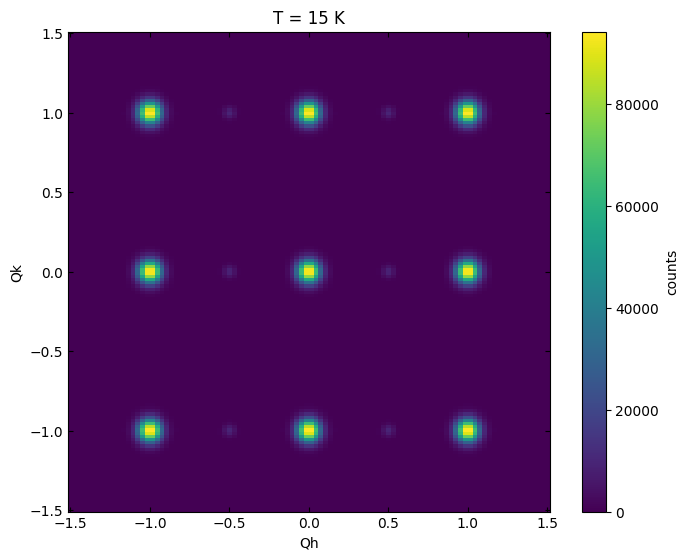
Clearly, we have some weak half integer reflections along H which are only present at low temperature.

Visualizing the phase transition

As a first step to parameterizing this phase transition, we can perform a linecut (learn more) that passes through the half-integer reflections.

xtl.cut_data(center=(0.0,0.0,0.0), window=(1.5,0.2,0.2))
xtl.plot_linecuts()

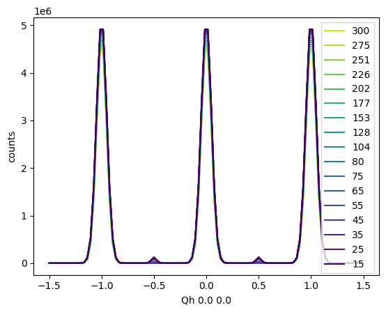
This plot of the linecut reveals the half integer peaks, but it’s hard to tell at exactly what temperature they turn on… To better visualize this, we can plot the linecuts as a heatmap in reciprocal space at various temperatures using the .plot_linecuts_heatmap() method.

xtl.plot_linecuts_heatmap(vmin=0, vmax=1.5e5)

<matplotlib.collections.QuadMesh at 0x739adc2c69b0>

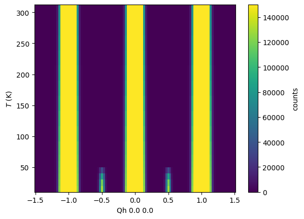
Here, it’s easier to see that the half integer peaks turn on at about T = 50 K, marking the phase transition temperature.

Fitting an order parameter

A more quantitative approach here is to combine this analysis with a fitting of the half-integer peaks, which will allow us to quantitatively track the order parameter by examining the temperature dependence of the peak parameters (e.g., peak height, peak width).

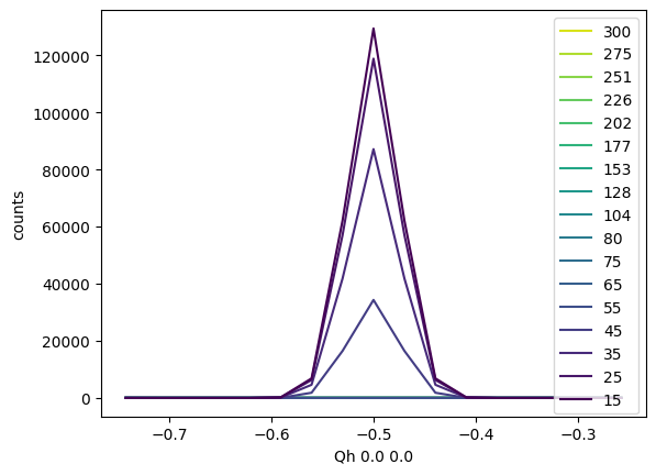
First, let’s narrow our linecut to only include a single half-integer reflection of interest.

xtl.cut_data(center=(-0.5,0.0,0.0), window=(0.25,0.2,0.2))
xtl.plot_linecuts()

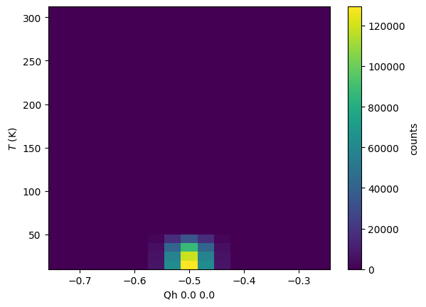
As above, we can also plot the heatmap version of the same plot, which allows us to clearly see the transition.

xtl.plot_linecuts_heatmap()

<matplotlib.collections.QuadMesh at 0x739a81cfee90>

Next, we can use the fitting tools in nxs_analysis_tools to fit these peaks (learn more).

from lmfit.models import GaussianModel, LinearModel

# Set the model components for the peak and background
xtl.set_model_components([GaussianModel(prefix='peak'), LinearModel(prefix='background')])

# Initialize the parameters for the model
xtl.make_params()

# Perform an initial guess
xtl.guess()

# Add in some helpful constraints
for T in xtl.temperatures:
    # Constrain the peak center to fall between -0.6 and -0.4 along H
    xtl.linecutmodels[T].params['peakcenter'].set(value=-0.5, min=-0.6, max=-0.4)
    # Constrain the peak amplitude to positive values
    xtl.linecutmodels[T].params['peakamplitude'].set(min=0)

# Perform the fitting procedure
xtl.fit()

# Optional: view the resulting fits
# xtl.plot_fit()

Fits completed.

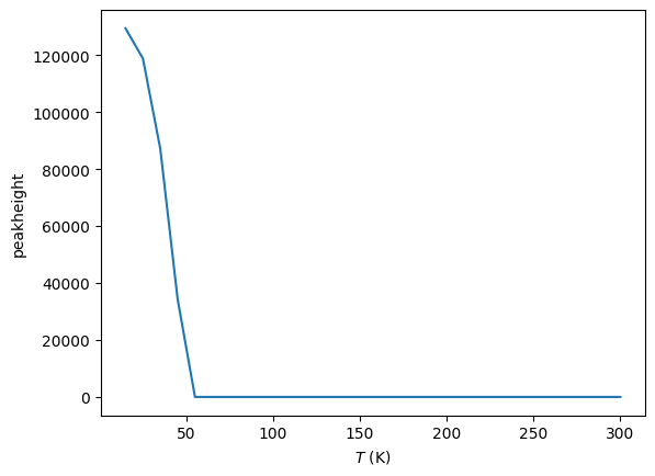
Now that the fits have been completed, we can use the .plot_order_parameter() method to plot the temperature dependence of a chosen parameter in the model (default peakheight) which gives us a good measure of the order parameter across the phase transition.

xtl.plot_order_parameter()

(<Figure size 640x480 with 1 Axes>,
 <Axes: xlabel='$T$ (K)', ylabel='peakheight'>)

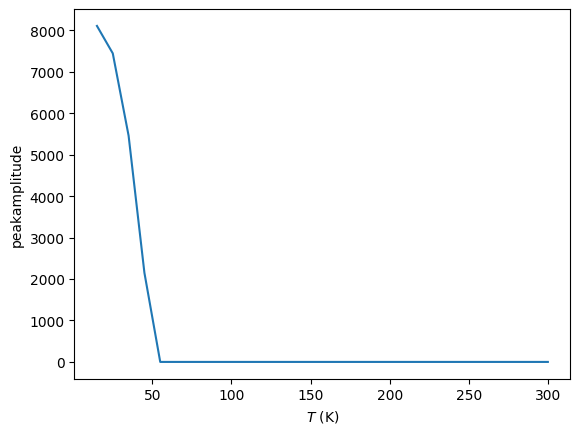
Use the argument param_name to select any other order parameter from the available model parameters.

xtl.plot_order_parameter(param_name='peakamplitude')

(<Figure size 640x480 with 1 Axes>,
 <Axes: xlabel='$T$ (K)', ylabel='peakamplitude'>)