Fitting linecuts using the lmfit package
Import functions
from nxs_analysis_tools.datareduction import load_transform, Scissors
from nxs_analysis_tools.fitting import LinecutModel
from nxs_analysis_tools.datasets import cubic

from lmfit.models import GaussianModel, LinearModel
import numpy as np
import matplotlib.pyplot as plt

# Download example data and save cache directory as sample_directory
sample_directory = cubic(temperatures=[15])
Load data
data = load_transform(f'{sample_directory}/cubic_15.nxs')
data:NXdata
  @axes = ['Qh', 'Qk', 'Ql']
  @signal = 'counts'
  Qh = float64(100)
  Qk = float64(150)
  Ql = float64(200)
  counts = float64(100x150x200)
Perform linecuts
s = Scissors(data=data)
linecut = s.cut_data(center=(0,0,0), window=(0.1,0.5,0.1))
The LinecutModel class
The workhorse of the fitting algorithm here is the LinecutModel class which wraps both the Model and ModelResult classes of the lmfit package, among other information.
lm = LinecutModel(data=linecut)
Create lmfit model
Use the .set_model_components() method to set the model to be used for fitting the linecut. The model_components parameter must be a Model, CompositeModel, or list of Model objects.
# Using a list of Model objects
lm.set_model_components([GaussianModel(prefix='peak'), LinearModel(prefix='background')])

# Using a CompositeModel
lm.set_model_components(GaussianModel(prefix='peak') + LinearModel(prefix='background'))
Upon setting the model, the .params attribute is initialized with a Parameters object which holds the parameters for all components of the model.
lm.params
| name | value | initial value | min | max | vary | expression |
|---|---|---|---|---|---|---|
| peakamplitude | 1.00000000 | None | -inf | inf | True | |
| peakcenter | 0.00000000 | None | -inf | inf | True | |
| peaksigma | 1.00000000 | None | 0.00000000 | inf | True | |
| backgroundslope | 1.00000000 | None | -inf | inf | True | |
| backgroundintercept | 0.00000000 | None | -inf | inf | True | |
| peakfwhm | 2.35482000 | None | -inf | inf | False | 2.3548200*peaksigma |
| peakheight | 0.39894230 | None | -inf | inf | False | 0.3989423*peakamplitude/max(1e-15, peaksigma) |
Performing an initial guess
Use the .guess() method to perform an initial guess, which will overwrite any changes made to the parameter values and constraints set in the .params attribute.
lm.guess()
[Parameters([('peakamplitude', <Parameter 'peakamplitude', value=482528.7250417659, bounds=[-inf:inf]>), ('peakcenter', <Parameter 'peakcenter', value=-7.401486830834377e-17, bounds=[-inf:inf]>), ('peaksigma', <Parameter 'peaksigma', value=0.05033557046979864, bounds=[0.0:inf]>), ('peakfwhm', <Parameter 'peakfwhm', value=0.11853120805369124, bounds=[-inf:inf], expr='2.3548200*peaksigma'>), ('peakheight', <Parameter 'peakheight', value=3824355.5717666983, bounds=[-inf:inf], expr='0.3989423*peakamplitude/max(1e-15, peaksigma)'>)]),
 Parameters([('backgroundslope', <Parameter 'backgroundslope', value=9.271792676819166e-11, bounds=[-inf:inf]>), ('backgroundintercept', <Parameter 'backgroundintercept', value=404986.4717240573, bounds=[-inf:inf]>)])]
To view the guessed initial values, we can inspect the .params attribute.
lm.params
| name | value | initial value | min | max | vary | expression |
|---|---|---|---|---|---|---|
| peakamplitude | 482528.725 | 482528.7250417659 | -inf | inf | True | |
| peakcenter | -7.4015e-17 | -7.401486830834377e-17 | -inf | inf | True | |
| peaksigma | 0.05033557 | 0.05033557046979864 | 0.00000000 | inf | True | |
| backgroundslope | 9.2718e-11 | 9.271792676819166e-11 | -inf | inf | True | |
| backgroundintercept | 404986.472 | 404986.4717240573 | -inf | inf | True | |
| peakfwhm | 0.11853121 | None | -inf | inf | False | 2.3548200*peaksigma |
| peakheight | 3824355.57 | None | -inf | inf | False | 0.3989423*peakamplitude/max(1e-15, peaksigma) |
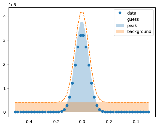
Visualize the initial guesses
lm.plot_initial_guess()
Set parameter constraints
All constraints are set by accessing the individiual parameters through the .params attribute. See https://lmfit.github.io/lmfit-py/constraints.html for more information on mathematical constraints allowed by lmfit.
# Constrain the peak amplitude to be positive
lm.params['peakamplitude'].set(min=0)

# Constrain the range of the peak center
lm.params['peakcenter'].set(min=-0.1, max=0.1)
If we inspect the .params attribute again, we should see that the constraints are implemented.
lm.params
| name | value | initial value | min | max | vary | expression |
|---|---|---|---|---|---|---|
| peakamplitude | 482528.725 | 482528.7250417659 | 0.00000000 | inf | True | |
| peakcenter | -7.4015e-17 | -7.401486830834377e-17 | -0.10000000 | 0.10000000 | True | |
| peaksigma | 0.05033557 | 0.05033557046979864 | 0.00000000 | inf | True | |
| backgroundslope | 9.2718e-11 | 9.271792676819166e-11 | -inf | inf | True | |
| backgroundintercept | 404986.472 | 404986.4717240573 | -inf | inf | True | |
| peakfwhm | 0.11853121 | None | -inf | inf | False | 2.3548200*peaksigma |
| peakheight | 3824355.57 | None | -inf | inf | False | 0.3989423*peakamplitude/max(1e-15, peaksigma) |
Perform the fit
The .fit() method here automatically assumes the parameter values and constraints currently stored in the .params attribute and feeds them to the .fit() method from lmfit.
lm.fit()
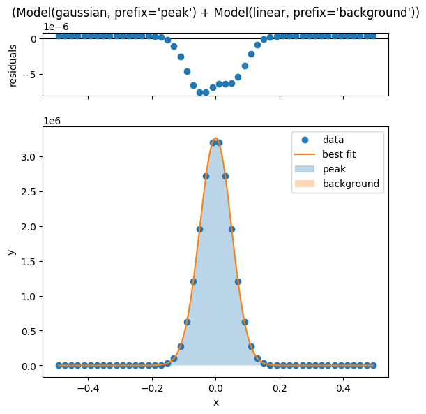
Visualize the fit
Once the fit is complete, we can visualize the fit and the residuals using the .plot_fit() method.
lm.plot_fit()

[[Model]]
    (Model(gaussian, prefix='peak') + Model(linear, prefix='background'))
[[Fit Statistics]]
    # fitting method   = leastsq
    # function evals   = 25
    # data points      = 50
    # variables        = 5
    chi-square         = 4.1415e-10
    reduced chi-square = 9.2033e-12
    Akaike info crit   = -1265.84087
    Bayesian info crit = -1256.28075
    R-squared          = 1.00000000
##  Warning: uncertainties could not be estimated:
    peakcenter:           at initial value
    backgroundslope:      at initial value
[[Variables]]
    peakamplitude:        407704.502 (init = 482528.7)
    peakcenter:          -1.7472e-14 (init = -7.401487e-17)
    peaksigma:            0.04987484 (init = 0.05033557)
    backgroundslope:      4.3073e-09 (init = 9.271793e-11)
    backgroundintercept: -4.3230e-07 (init = 404986.5)
    peakfwhm:             0.11744628 == '2.3548200*peaksigma'
    peakheight:           3261174.59 == '0.3989423*peakamplitude/max(1e-15, peaksigma)'
<Axes: xlabel='x', ylabel='y'>
The number of x values used to evaluate the fit curve can be set using the numpoints parameter, and any keyword arguments here will be passed to the .plot() method of the underlying ModelResult object.
lm.plot_fit(numpoints=1000)
[[Model]]
    (Model(gaussian, prefix='peak') + Model(linear, prefix='background'))
[[Fit Statistics]]
    # fitting method   = leastsq
    # function evals   = 25
    # data points      = 50
    # variables        = 5
    chi-square         = 4.1415e-10
    reduced chi-square = 9.2033e-12
    Akaike info crit   = -1265.84087
    Bayesian info crit = -1256.28075
    R-squared          = 1.00000000
##  Warning: uncertainties could not be estimated:
    peakcenter:           at initial value
    backgroundslope:      at initial value
[[Variables]]
    peakamplitude:        407704.502 (init = 482528.7)
    peakcenter:          -1.7472e-14 (init = -7.401487e-17)
    peaksigma:            0.04987484 (init = 0.05033557)
    backgroundslope:      4.3073e-09 (init = 9.271793e-11)
    backgroundintercept: -4.3230e-07 (init = 404986.5)
    peakfwhm:             0.11744628 == '2.3548200*peaksigma'
    peakheight:           3261174.59 == '0.3989423*peakamplitude/max(1e-15, peaksigma)'
<Axes: xlabel='x', ylabel='y'>
Access the fit values
The x and y values of the fit are stored in the .x (identical to the raw x values) and the .y_fit attributes.
lm.x
array([-0.493289, -0.473154, -0.45302 , ...,  0.45302 ,  0.473154,
        0.493289], shape=(50,))
lm.y_fit
array([-4.344241e-07, -4.343373e-07, -4.342467e-07, ..., -4.303441e-07,
       -4.302613e-07, -4.301746e-07], shape=(50,))
The residuals are stored within the ModelResult class of the lmfit package, which is stored in the .modelresult attribute of the LinecutModel class.
lm.modelresult.residual
array([4.344241e-07, 4.343374e-07, 4.342507e-07, ..., 4.303481e-07,
       4.302614e-07, 4.301746e-07], shape=(50,))
If .plot_fit() has already been called, then the evaluated data composing the fit curve can be found in .x_eval and .y_eval.
lm.x_eval
array([-0.493289, -0.492301, -0.491313, ...,  0.491313,  0.492301,
        0.493289], shape=(1000,))
lm.y_eval
array([-4.344241e-07, -4.344198e-07, -4.344156e-07, ..., -4.301832e-07,
       -4.301789e-07, -4.301746e-07], shape=(1000,))
If .plot_fit() has not been called, then evaluating the fit can be done in the standard lmfit way through the ModelResult object for either the total model or its individual components.
# Evaulate the total model
lm.modelresult.eval(x=np.linspace(-0.5,0.5,1000))
array([-4.344530e-07, -4.344487e-07, -4.344444e-07, ..., -4.301544e-07,
       -4.301500e-07, -4.301457e-07], shape=(1000,))
# Evaulate only the background component
lm.modelresult.components[1].eval(x=np.linspace(-0.5,0.5,1000))
array([-0.5     , -0.498999, -0.497998, ...,  0.497998,  0.498999,
        0.5     ], shape=(1000,))
You may also opt to evaluate all components at the same time, but separated by their individual contribution.
# Evaluate all components separately
evaluated_components = lm.modelresult.eval_components(x=np.linspace(-0.5,0.5,1000))
Using this approach, a dict is generated where the contribution of each component is labeled by its prefix.
evaluated_components
{'peak': array([4.892499e-16, 5.981719e-16, 7.310488e-16, ..., 7.310488e-16,
        5.981719e-16, 4.892499e-16], shape=(1000,)),
 'background': array([-4.344530e-07, -4.344487e-07, -4.344444e-07, ..., -4.301544e-07,
        -4.301501e-07, -4.301457e-07], shape=(1000,))}
evaluated_components['peak']
array([4.892499e-16, 5.981719e-16, 7.310488e-16, ..., 7.310488e-16,
       5.981719e-16, 4.892499e-16], shape=(1000,))
evaluated_components['background']
array([-4.344530e-07, -4.344487e-07, -4.344444e-07, ..., -4.301544e-07,
       -4.301501e-07, -4.301457e-07], shape=(1000,))
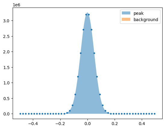
These can then be plotted together to show their individual contributions. See below for an example.
plt.plot(lm.x, lm.y, '.')
plt.fill_between(np.linspace(-0.5,0.5,1000), evaluated_components['peak'], alpha=0.5, label='peak')
plt.fill_between(np.linspace(-0.5,0.5,1000), evaluated_components['background'], alpha=0.5, label='background')
plt.legend()
<matplotlib.legend.Legend at 0x7608b538af50>
Viewing the fit report
lm.print_fit_report()
[[Model]]
    (Model(gaussian, prefix='peak') + Model(linear, prefix='background'))
[[Fit Statistics]]
    # fitting method   = leastsq
    # function evals   = 25
    # data points      = 50
    # variables        = 5
    chi-square         = 4.1415e-10
    reduced chi-square = 9.2033e-12
    Akaike info crit   = -1265.84087
    Bayesian info crit = -1256.28075
    R-squared          = 1.00000000
##  Warning: uncertainties could not be estimated:
    peakcenter:           at initial value
    backgroundslope:      at initial value
[[Variables]]
    peakamplitude:        407704.502 (init = 482528.7)
    peakcenter:          -1.7472e-14 (init = -7.401487e-17)
    peaksigma:            0.04987484 (init = 0.05033557)
    backgroundslope:      4.3073e-09 (init = 9.271793e-11)
    backgroundintercept: -4.3230e-07 (init = 404986.5)
    peakfwhm:             0.11744628 == '2.3548200*peaksigma'
    peakheight:           3261174.59 == '0.3989423*peakamplitude/max(1e-15, peaksigma)'
Performing a simple linecut with no customization
The .fit_peak_simple() method offers a quick but rudimentary way to fit a peak, using a pseudo-Voigt peak shape with a linear background.
lm.fit_peak_simple()
lm.plot_fit()
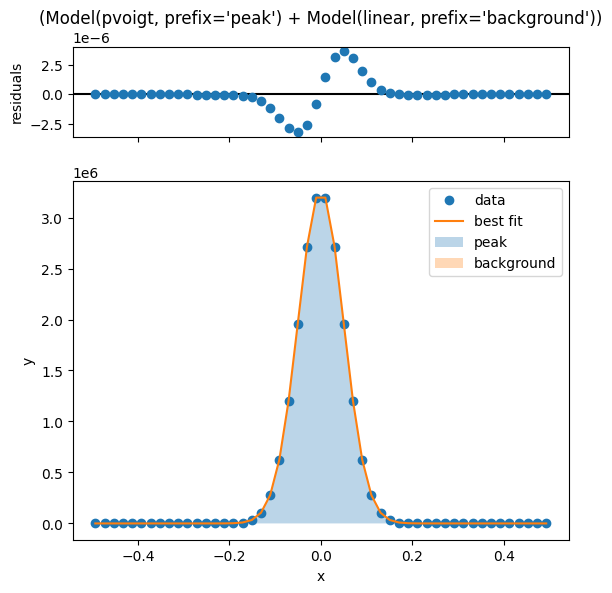
[[Model]]
    (Model(pvoigt, prefix='peak') + Model(linear, prefix='background'))
[[Fit Statistics]]
    # fitting method   = leastsq
    # function evals   = 239
    # data points      = 50
    # variables        = 6
    chi-square         = 7.1310e-11
    reduced chi-square = 1.6207e-12
    Akaike info crit   = -1351.80009
    Bayesian info crit = -1340.32795
    R-squared          = 1.00000000
##  Warning: uncertainties could not be estimated:
    peakcenter:           at initial value
    peakfraction:         at boundary
    backgroundslope:      at initial value
[[Variables]]
    peakamplitude:        407704.502 (init = 603160.9)
    peakcenter:          -8.6824e-14 (init = -7.401487e-17)
    peaksigma:            0.05872314 (init = 0.05033557)
    peakfraction:         3.0309e-13 (init = 0.5)
    peakfwhm:             0.11744628 == '2.0000000*peaksigma'
    peakheight:           3261174.43 == '(((1-peakfraction)*peakamplitude)/max(1e-15, (peaksigma*sqrt(pi/log(2))))+(peakfraction*peakamplitude)/max(1e-15, (pi*peaksigma)))'
    backgroundslope:      9.0210e-17 (init = 9.271793e-11)
    backgroundintercept: -9.1841e-12 (init = 404986.5)
<Axes: xlabel='x', ylabel='y'>