Fitting CHESS temperature dependent linecuts
Import functions
from nxs_analysis_tools.datareduction import load_data, Scissors
from nxs_analysis_tools.chess import *
from nxs_analysis_tools.datasets import cubic

from lmfit.models import GaussianModel, LinearModel

# Load example datasets and store cache directory
sample_directory = cubic()
Create TempDependence object and load data
sample = TempDependence(sample_directory)
sample.load_transforms()
# Or, load_datasets() if using legacy CHESS data format
data:NXdata
  @axes = ['Qh', 'Qk', 'Ql']
  @signal = 'counts'
  Qh = float64(100)
  Qk = float64(150)
  Ql = float64(200)
  counts = float64(100x150x200)
data:NXdata
  @axes = ['Qh', 'Qk', 'Ql']
  @signal = 'counts'
  Qh = float64(100)
  Qk = float64(150)
  Ql = float64(200)
  counts = float64(100x150x200)
data:NXdata
  @axes = ['Qh', 'Qk', 'Ql']
  @signal = 'counts'
  Qh = float64(100)
  Qk = float64(150)
  Ql = float64(200)
  counts = float64(100x150x200)
data:NXdata
  @axes = ['Qh', 'Qk', 'Ql']
  @signal = 'counts'
  Qh = float64(100)
  Qk = float64(150)
  Ql = float64(200)
  counts = float64(100x150x200)
data:NXdata
  @axes = ['Qh', 'Qk', 'Ql']
  @signal = 'counts'
  Qh = float64(100)
  Qk = float64(150)
  Ql = float64(200)
  counts = float64(100x150x200)
data:NXdata
  @axes = ['Qh', 'Qk', 'Ql']
  @signal = 'counts'
  Qh = float64(100)
  Qk = float64(150)
  Ql = float64(200)
  counts = float64(100x150x200)
data:NXdata
  @axes = ['Qh', 'Qk', 'Ql']
  @signal = 'counts'
  Qh = float64(100)
  Qk = float64(150)
  Ql = float64(200)
  counts = float64(100x150x200)
data:NXdata
  @axes = ['Qh', 'Qk', 'Ql']
  @signal = 'counts'
  Qh = float64(100)
  Qk = float64(150)
  Ql = float64(200)
  counts = float64(100x150x200)
data:NXdata
  @axes = ['Qh', 'Qk', 'Ql']
  @signal = 'counts'
  Qh = float64(100)
  Qk = float64(150)
  Ql = float64(200)
  counts = float64(100x150x200)
data:NXdata
  @axes = ['Qh', 'Qk', 'Ql']
  @signal = 'counts'
  Qh = float64(100)
  Qk = float64(150)
  Ql = float64(200)
  counts = float64(100x150x200)
data:NXdata
  @axes = ['Qh', 'Qk', 'Ql']
  @signal = 'counts'
  Qh = float64(100)
  Qk = float64(150)
  Ql = float64(200)
  counts = float64(100x150x200)
data:NXdata
  @axes = ['Qh', 'Qk', 'Ql']
  @signal = 'counts'
  Qh = float64(100)
  Qk = float64(150)
  Ql = float64(200)
  counts = float64(100x150x200)
data:NXdata
  @axes = ['Qh', 'Qk', 'Ql']
  @signal = 'counts'
  Qh = float64(100)
  Qk = float64(150)
  Ql = float64(200)
  counts = float64(100x150x200)
data:NXdata
  @axes = ['Qh', 'Qk', 'Ql']
  @signal = 'counts'
  Qh = float64(100)
  Qk = float64(150)
  Ql = float64(200)
  counts = float64(100x150x200)
data:NXdata
  @axes = ['Qh', 'Qk', 'Ql']
  @signal = 'counts'
  Qh = float64(100)
  Qk = float64(150)
  Ql = float64(200)
  counts = float64(100x150x200)
data:NXdata
  @axes = ['Qh', 'Qk', 'Ql']
  @signal = 'counts'
  Qh = float64(100)
  Qk = float64(150)
  Ql = float64(200)
  counts = float64(100x150x200)
data:NXdata
  @axes = ['Qh', 'Qk', 'Ql']
  @signal = 'counts'
  Qh = float64(100)
  Qk = float64(150)
  Ql = float64(200)
  counts = float64(100x150x200)
Perform linecuts
sample.cut_data(center=(0,0,0), window=(0.1,0.5,0.1))
{'15': NXdata('data'),
 '25': NXdata('data'),
 '35': NXdata('data'),
 '45': NXdata('data'),
 '55': NXdata('data'),
 '65': NXdata('data'),
 '75': NXdata('data'),
 '80': NXdata('data'),
 '104': NXdata('data'),
 '128': NXdata('data'),
 '153': NXdata('data'),
 '177': NXdata('data'),
 '202': NXdata('data'),
 '226': NXdata('data'),
 '251': NXdata('data'),
 '275': NXdata('data'),
 '300': NXdata('data')}
The LinecutModel class
Each TempDependence object has a LinecutModel for each temperature, stored in the .linecutmodels attribute. When a linecut is performed using the .cut_data() method, these are automatically initialized with the x and y data from the linecut.
sample.linecutmodels
{'15': <nxs_analysis_tools.fitting.LinecutModel at 0x72bd308eeaa0>,
 '25': <nxs_analysis_tools.fitting.LinecutModel at 0x72bd308ee9e0>,
 '35': <nxs_analysis_tools.fitting.LinecutModel at 0x72bd308eea70>,
 '45': <nxs_analysis_tools.fitting.LinecutModel at 0x72bd308eeb60>,
 '55': <nxs_analysis_tools.fitting.LinecutModel at 0x72bd308eeb90>,
 '65': <nxs_analysis_tools.fitting.LinecutModel at 0x72bd308eebf0>,
 '75': <nxs_analysis_tools.fitting.LinecutModel at 0x72bd308eec80>,
 '80': <nxs_analysis_tools.fitting.LinecutModel at 0x72bd308eed40>,
 '104': <nxs_analysis_tools.fitting.LinecutModel at 0x72bd308eeda0>,
 '128': <nxs_analysis_tools.fitting.LinecutModel at 0x72bd308eee00>,
 '153': <nxs_analysis_tools.fitting.LinecutModel at 0x72bd308eee60>,
 '177': <nxs_analysis_tools.fitting.LinecutModel at 0x72bd308eeec0>,
 '202': <nxs_analysis_tools.fitting.LinecutModel at 0x72bd308eef20>,
 '226': <nxs_analysis_tools.fitting.LinecutModel at 0x72bd308eef80>,
 '251': <nxs_analysis_tools.fitting.LinecutModel at 0x72bd308eefe0>,
 '275': <nxs_analysis_tools.fitting.LinecutModel at 0x72bd308ef040>,
 '300': <nxs_analysis_tools.fitting.LinecutModel at 0x72bd308ef0a0>}
Create lmfit model
Use the .set_model_components() method to set the model to be used for fitting the linecut. The model_components parameter must be a Model, CompositeModel, or list of Model objects.
# Using a list of Model objects
sample.set_model_components([GaussianModel(prefix='peak'), LinearModel(prefix='background')])

# Using a CompositeModel
sample.set_model_components(GaussianModel(prefix='peak') + LinearModel(prefix='background'))
Upon setting the model, the .params attribute of each LinecutModel is initialized with a Parameters object which holds the parameters for all components of the model.
sample.linecutmodels['15'].params
| name | value | initial value | min | max | vary | expression |
|---|---|---|---|---|---|---|
| peakamplitude | 1.00000000 | None | -inf | inf | True | |
| peakcenter | 0.00000000 | None | -inf | inf | True | |
| peaksigma | 1.00000000 | None | 0.00000000 | inf | True | |
| backgroundslope | 1.00000000 | None | -inf | inf | True | |
| backgroundintercept | 0.00000000 | None | -inf | inf | True | |
| peakfwhm | 2.35482000 | None | -inf | inf | False | 2.3548200*peaksigma |
| peakheight | 0.39894230 | None | -inf | inf | False | 0.3989423*peakamplitude/max(1e-15, peaksigma) |
Performing an initial guess
Use the .guess() method to perform an initial guess, which will overwrite any changes made to the parameter values and constraints set in the .params attribute.
sample.guess()
To view the guessed initial values, we can inspect the .params attribute for any given dataset.
sample.linecutmodels['15'].params
| name | value | initial value | min | max | vary | expression |
|---|---|---|---|---|---|---|
| peakamplitude | 482528.725 | 482528.7250417659 | -inf | inf | True | |
| peakcenter | -7.4015e-17 | -7.401486830834377e-17 | -inf | inf | True | |
| peaksigma | 0.05033557 | 0.05033557046979864 | 0.00000000 | inf | True | |
| backgroundslope | 9.2718e-11 | 9.271792676819166e-11 | -inf | inf | True | |
| backgroundintercept | 404986.472 | 404986.4717240573 | -inf | inf | True | |
| peakfwhm | 0.11853121 | None | -inf | inf | False | 2.3548200*peaksigma |
| peakheight | 3824355.57 | None | -inf | inf | False | 0.3989423*peakamplitude/max(1e-15, peaksigma) |
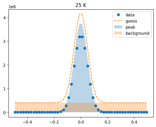
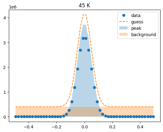
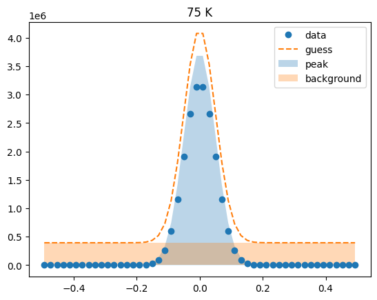
Visualize the initial guesses
sample.plot_initial_guess()


Set parameter constraints
All constraints are set by accessing the individiual parameters through the .params attribute. See https://lmfit.github.io/lmfit-py/constraints.html for more information on mathematical constraints allowed by lmfit.
# Constrain the peak amplitude to be positive
sample.linecutmodels['15'].params['peakamplitude'].set(min=0)

# Constrain the range of the peak center
sample.linecutmodels['15'].params['peakcenter'].set(min=-0.1, max=0.1)
If we inspect the .params attribute again, we should see that the constraints are implemented.
sample.linecutmodels['15'].params
| name | value | initial value | min | max | vary | expression |
|---|---|---|---|---|---|---|
| peakamplitude | 482528.725 | 482528.7250417659 | 0.00000000 | inf | True | |
| peakcenter | -7.4015e-17 | -7.401486830834377e-17 | -0.10000000 | 0.10000000 | True | |
| peaksigma | 0.05033557 | 0.05033557046979864 | 0.00000000 | inf | True | |
| backgroundslope | 9.2718e-11 | 9.271792676819166e-11 | -inf | inf | True | |
| backgroundintercept | 404986.472 | 404986.4717240573 | -inf | inf | True | |
| peakfwhm | 0.11853121 | None | -inf | inf | False | 2.3548200*peaksigma |
| peakheight | 3824355.57 | None | -inf | inf | False | 0.3989423*peakamplitude/max(1e-15, peaksigma) |
It is practical in many cases to set a constraint for all datasets at once, since they are likely to have very similar data. For example, we may wish to constrain the peak center to range between -0.1 and 0.1 at all temperatures, with an initial value of 0.05.
Rather than accessing each temperature manually, we can use the .params_set() method of the TempDependence object to set a constraint on all the LinecutModel objects at once.
sample.params_set(name='peakcenter', value=0.05, min=-0.1, max=0.1)
Now, we can examine the individual parameters of any LinecutModel and find that the constraint has been applied.
sample.linecutmodels['300'].params
| name | value | initial value | min | max | vary | expression |
|---|---|---|---|---|---|---|
| peakamplitude | 441104.184 | 441104.18388416775 | -inf | inf | True | |
| peakcenter | 0.05000000 | 0.05 | -0.10000000 | 0.10000000 | True | |
| peaksigma | 0.05033557 | 0.05033557046979864 | 0.00000000 | inf | True | |
| backgroundslope | 8.3374e-11 | 8.33739637361666e-11 | -inf | inf | True | |
| backgroundintercept | 352859.729 | 352859.7293307577 | -inf | inf | True | |
| peakfwhm | 0.11853121 | None | -inf | inf | False | 2.3548200*peaksigma |
| peakheight | 3496039.00 | None | -inf | inf | False | 0.3989423*peakamplitude/max(1e-15, peaksigma) |
Perform the fit
The .fit() method here automatically assumes the parameter values and constraints currently stored in the .params attribute of each model, and feeds them to the .fit() method from lmfit.
sample.fit()
Fits completed.
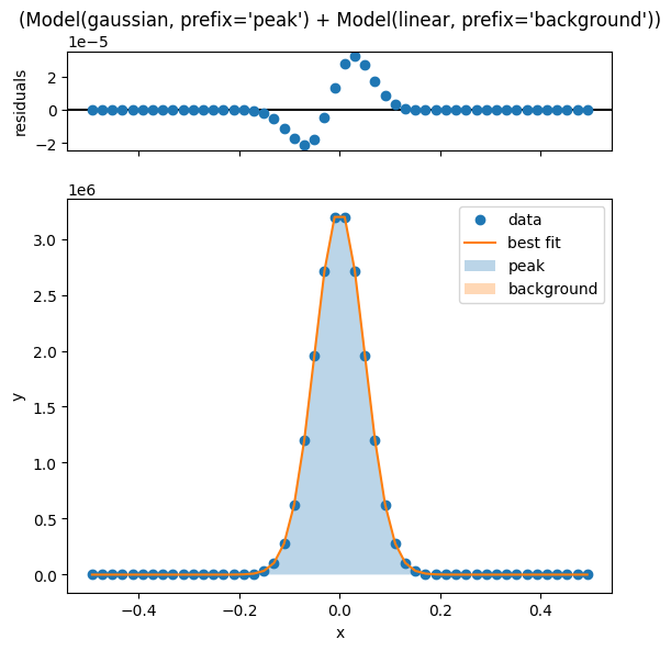
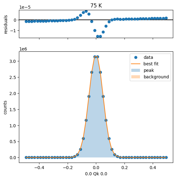
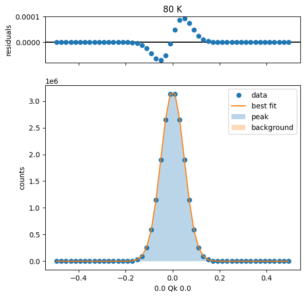
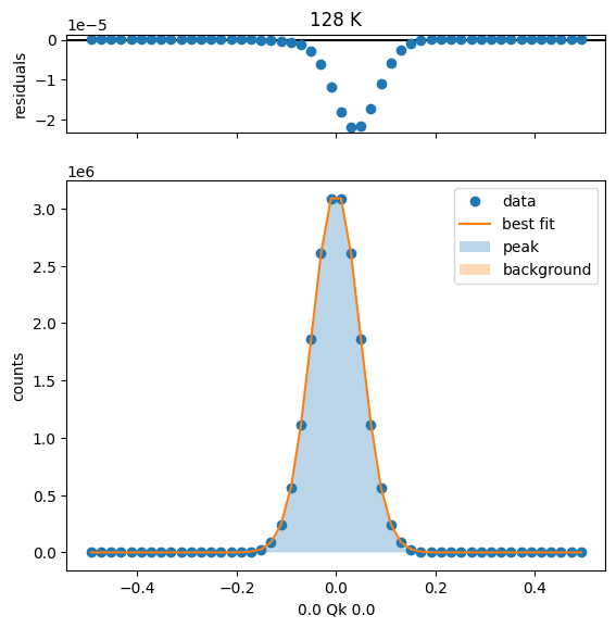
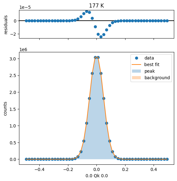
Visualize the fits
Once the fit is complete, we can visualize the fit and the residuals using the .plot_fit() method of each LinecutModel.
sample.linecutmodels['15'].plot_fit()
[[Model]]
    (Model(gaussian, prefix='peak') + Model(linear, prefix='background'))
[[Fit Statistics]]
    # fitting method   = leastsq
    # function evals   = 37
    # data points      = 50
    # variables        = 5
    chi-square         = 4.4542e-09
    reduced chi-square = 9.8983e-11
    Akaike info crit   = -1147.07151
    Bayesian info crit = -1137.51140
    R-squared          = 1.00000000
[[Variables]]
    peakamplitude:        407704.502 +/- 8.4625e-07 (0.00%) (init = 482528.7)
    peakcenter:          -5.6972e-13 +/- 1.0295e-13 (18.07%) (init = 0.05)
    peaksigma:            0.04987484 +/- 1.0870e-13 (0.00%) (init = 0.05033557)
    backgroundslope:     -1.7676e-11 +/- 5.1870e-06 (29343894.48%) (init = 9.271793e-11)
    backgroundintercept: -2.3391e-07 +/- 1.6398e-06 (701.07%) (init = 404986.5)
    peakfwhm:             0.11744628 +/- 2.5597e-13 (0.00%) == '2.3548200*peaksigma'
    peakheight:           3261174.59 +/- 5.9249e-06 (0.00%) == '0.3989423*peakamplitude/max(1e-15, peaksigma)'
[[Correlations]] (unreported correlations are < 0.100)
    C(peakamplitude, peaksigma)           = +0.6364
    C(peakamplitude, backgroundintercept) = -0.5118
    C(peaksigma, backgroundintercept)     = -0.3278
<Axes: xlabel='x', ylabel='y'>
Visualize all fits
The .plot_fit() method of the TempDependence object prints fit results for all temperatures. The parameter fit_report (default True) determines whether the fit report is also printed.
Additionally, an optional Markdown heading can be displayed using the mdheadings parameter (default False).
sample.plot_fit(mdheadings=True)
15 K Fit Results

[[Model]]
    (Model(gaussian, prefix='peak') + Model(linear, prefix='background'))
[[Fit Statistics]]
    # fitting method   = leastsq
    # function evals   = 37
    # data points      = 50
    # variables        = 5
    chi-square         = 4.4542e-09
    reduced chi-square = 9.8983e-11
    Akaike info crit   = -1147.07151
    Bayesian info crit = -1137.51140
    R-squared          = 1.00000000
[[Variables]]
    peakamplitude:        407704.502 +/- 8.4625e-07 (0.00%) (init = 482528.7)
    peakcenter:          -5.6972e-13 +/- 1.0295e-13 (18.07%) (init = 0.05)
    peaksigma:            0.04987484 +/- 1.0870e-13 (0.00%) (init = 0.05033557)
    backgroundslope:     -1.7676e-11 +/- 5.1870e-06 (29343894.48%) (init = 9.271793e-11)
    backgroundintercept: -2.3391e-07 +/- 1.6398e-06 (701.07%) (init = 404986.5)
    peakfwhm:             0.11744628 +/- 2.5597e-13 (0.00%) == '2.3548200*peaksigma'
    peakheight:           3261174.59 +/- 5.9249e-06 (0.00%) == '0.3989423*peakamplitude/max(1e-15, peaksigma)'
[[Correlations]] (unreported correlations are < 0.100)
    C(peakamplitude, peaksigma)           = +0.6364
    C(peakamplitude, backgroundintercept) = -0.5118
    C(peaksigma, backgroundintercept)     = -0.3278
[[Model]]
    (Model(gaussian, prefix='peak') + Model(linear, prefix='background'))
[[Fit Statistics]]
    # fitting method   = leastsq
    # function evals   = 37
    # data points      = 50
    # variables        = 5
    chi-square         = 3.9440e-08
    reduced chi-square = 8.7645e-10
    Akaike info crit   = -1038.02503
    Bayesian info crit = -1028.46492
    R-squared          = 1.00000000
[[Variables]]
    peakamplitude:        405849.455 +/- 2.5177e-06 (0.00%) (init = 481106.9)
    peakcenter:          -1.9756e-12 +/- 3.0881e-13 (15.63%) (init = 0.05)
    peaksigma:            0.04979123 +/- 3.2391e-13 (0.00%) (init = 0.05033557)
    backgroundslope:      1.6829e-10 +/- 1.5502e-05 (9211309.16%) (init = 9.206435e-11)
    backgroundintercept:  7.0271e-07 +/- 4.8768e-06 (694.00%) (init = 403143.8)
    peakfwhm:             0.11724939 +/- 7.6274e-13 (0.00%) == '2.3548200*peaksigma'
    peakheight:           3251787.76 +/- 1.7658e-05 (0.00%) == '0.3989423*peakamplitude/max(1e-15, peaksigma)'
[[Correlations]] (unreported correlations are < 0.100)
    C(peakamplitude, peaksigma)           = +0.6358
    C(peakamplitude, backgroundintercept) = -0.5128
    C(peaksigma, backgroundintercept)     = -0.3260
[[Model]]
    (Model(gaussian, prefix='peak') + Model(linear, prefix='background'))
[[Fit Statistics]]
    # fitting method   = leastsq
    # function evals   = 37
    # data points      = 50
    # variables        = 5
    chi-square         = 2.3783e-08
    reduced chi-square = 5.2850e-10
    Akaike info crit   = -1063.31666
    Bayesian info crit = -1053.75654
    R-squared          = 1.00000000
[[Variables]]
    peakamplitude:        403995.273 +/- 1.9528e-06 (0.00%) (init = 479682.7)
    peakcenter:          -1.5850e-12 +/- 2.3985e-13 (15.13%) (init = 0.05)
    peaksigma:            0.04970748 +/- 2.5239e-13 (0.00%) (init = 0.05033557)
    backgroundslope:      1.4944e-10 +/- 1.2066e-05 (8074472.07%) (init = 8.948964e-11)
    backgroundintercept: -5.6968e-07 +/- 3.7885e-06 (665.03%) (init = 401302)
    peakfwhm:             0.11705216 +/- 5.9433e-13 (0.00%) == '2.3548200*peaksigma'
    peakheight:           3242385.47 +/- 1.3709e-05 (0.00%) == '0.3989423*peakamplitude/max(1e-15, peaksigma)'
[[Correlations]] (unreported correlations are < 0.100)
    C(peakamplitude, peaksigma)           = +0.6370
    C(peakamplitude, backgroundintercept) = -0.5123
    C(peaksigma, backgroundintercept)     = -0.3298
[[Model]]
    (Model(gaussian, prefix='peak') + Model(linear, prefix='background'))
[[Fit Statistics]]
    # fitting method   = leastsq
    # function evals   = 37
    # data points      = 50
    # variables        = 5
    chi-square         = 5.4343e-08
    reduced chi-square = 1.2076e-09
    Akaike info crit   = -1021.99892
    Bayesian info crit = -1012.43881
    R-squared          = 1.00000000
[[Variables]]
    peakamplitude:        402141.971 +/- 2.9455e-06 (0.00%) (init = 478256.3)
    peakcenter:           2.3830e-12 +/- 3.5747e-13 (15.00%) (init = 0.05)
    peaksigma:            0.04962358 +/- 3.8166e-13 (0.00%) (init = 0.05033557)
    backgroundslope:     -6.1735e-11 +/- 1.7927e-05 (29038232.24%) (init = 8.969425e-11)
    backgroundintercept:  7.0822e-07 +/- 5.7205e-06 (807.73%) (init = 399461)
    peakfwhm:             0.11685461 +/- 8.9873e-13 (0.00%) == '2.3548200*peaksigma'
    peakheight:           3232967.73 +/- 2.0753e-05 (0.00%) == '0.3989423*peakamplitude/max(1e-15, peaksigma)'
[[Correlations]] (unreported correlations are < 0.100)
    C(peakamplitude, peaksigma)           = +0.6355
    C(peakamplitude, backgroundintercept) = -0.5104
    C(peaksigma, backgroundintercept)     = -0.3251
[[Model]]
    (Model(gaussian, prefix='peak') + Model(linear, prefix='background'))
[[Fit Statistics]]
    # fitting method   = leastsq
    # function evals   = 37
    # data points      = 50
    # variables        = 5
    chi-square         = 7.4821e-10
    reduced chi-square = 1.6627e-11
    Akaike info crit   = -1236.26814
    Bayesian info crit = -1226.70803
    R-squared          = 1.00000000
[[Variables]]
    peakamplitude:        400289.564 +/- 3.4600e-07 (0.00%) (init = 476827.5)
    peakcenter:          -2.6987e-13 +/- 4.2480e-14 (15.74%) (init = 0.05)
    peaksigma:            0.04953955 +/- 4.4888e-14 (0.00%) (init = 0.05033557)
    backgroundslope:     -6.0345e-11 +/- 2.1292e-06 (3528309.34%) (init = 9.27811e-11)
    backgroundintercept:  7.4672e-08 +/- 6.7120e-07 (898.87%) (init = 397621)
    peakfwhm:             0.11665671 +/- 1.0570e-13 (0.00%) == '2.3548200*peaksigma'
    peakheight:           3223534.55 +/- 2.4388e-06 (0.00%) == '0.3989423*peakamplitude/max(1e-15, peaksigma)'
[[Correlations]] (unreported correlations are < 0.100)
    C(peakamplitude, peaksigma)           = +0.6357
    C(peakamplitude, backgroundintercept) = -0.5132
    C(peaksigma, backgroundintercept)     = -0.3259
[[Model]]
    (Model(gaussian, prefix='peak') + Model(linear, prefix='background'))
[[Fit Statistics]]
    # fitting method   = leastsq
    # function evals   = 37
    # data points      = 50
    # variables        = 5
    chi-square         = 2.0580e-09
    reduced chi-square = 4.5734e-11
    Akaike info crit   = -1185.67693
    Bayesian info crit = -1176.11682
    R-squared          = 1.00000000
[[Variables]]
    peakamplitude:        398438.067 +/- 5.7190e-07 (0.00%) (init = 475396.4)
    peakcenter:           3.1823e-13 +/- 7.0444e-14 (22.14%) (init = 0.05)
    peaksigma:            0.04945537 +/- 7.4617e-14 (0.00%) (init = 0.05033557)
    backgroundslope:      1.0843e-10 +/- 2.1186e-06 (1953914.73%) (init = 8.492314e-11)
    backgroundintercept: -2.2079e-07 +/- 1.1129e-06 (504.06%) (init = 395781.8)
    peakfwhm:             0.11645849 +/- 1.7571e-13 (0.00%) == '2.3548200*peaksigma'
    peakheight:           3214085.92 +/- 4.0431e-06 (0.00%) == '0.3989423*peakamplitude/max(1e-15, peaksigma)'
[[Correlations]] (unreported correlations are < 0.100)
    C(peakamplitude, peaksigma)           = +0.6359
    C(peakamplitude, backgroundintercept) = -0.5095
    C(peaksigma, backgroundintercept)     = -0.3264
[[Model]]
    (Model(gaussian, prefix='peak') + Model(linear, prefix='background'))
[[Fit Statistics]]
    # fitting method   = leastsq
    # function evals   = 37
    # data points      = 50
    # variables        = 5
    chi-square         = 9.8721e-10
    reduced chi-square = 2.1938e-11
    Akaike info crit   = -1222.40793
    Bayesian info crit = -1212.84781
    R-squared          = 1.00000000
[[Variables]]
    peakamplitude:        396587.494 +/- 3.9597e-07 (0.00%) (init = 473963)
    peakcenter:           2.1952e-13 +/- 4.9058e-14 (22.35%) (init = 0.05)
    peaksigma:            0.04937104 +/- 5.1737e-14 (0.00%) (init = 0.05033557)
    backgroundslope:     -3.1995e-06 +/- 2.2726e-06 (71.03%) (init = 9.308819e-11)
    backgroundintercept: -1.6757e-07 +/- 7.7031e-07 (459.70%) (init = 393943.6)
    peakfwhm:             0.11625992 +/- 1.2183e-13 (0.00%) == '2.3548200*peaksigma'
    peakheight:           3204621.85 +/- 2.8052e-06 (0.00%) == '0.3989423*peakamplitude/max(1e-15, peaksigma)'
[[Correlations]] (unreported correlations are < 0.100)
    C(peakamplitude, peaksigma)           = +0.6350
    C(peakamplitude, backgroundintercept) = -0.5103
    C(peaksigma, backgroundintercept)     = -0.3237
[[Model]]
    (Model(gaussian, prefix='peak') + Model(linear, prefix='background'))
[[Fit Statistics]]
    # fitting method   = leastsq
    # function evals   = 37
    # data points      = 50
    # variables        = 5
    chi-square         = 4.0817e-08
    reduced chi-square = 9.0704e-10
    Akaike info crit   = -1036.31003
    Bayesian info crit = -1026.74991
    R-squared          = 1.00000000
[[Variables]]
    peakamplitude:        395662.559 +/- 2.5491e-06 (0.00%) (init = 473245.4)
    peakcenter:          -2.0652e-12 +/- 3.1738e-13 (15.37%) (init = 0.05)
    peaksigma:            0.04932883 +/- 3.3349e-13 (0.00%) (init = 0.05033557)
    backgroundslope:     -2.0195e-07 +/- 6.6918e-06 (3313.63%) (init = 8.835303e-11)
    backgroundintercept:  1.3057e-07 +/- 5.0051e-06 (3833.27%) (init = 393024.8)
    peakfwhm:             0.11616051 +/- 7.8531e-13 (0.00%) == '2.3548200*peaksigma'
    peakheight:           3199884.04 +/- 1.8042e-05 (0.00%) == '0.3989423*peakamplitude/max(1e-15, peaksigma)'
[[Correlations]] (unreported correlations are < 0.100)
    C(peakamplitude, peaksigma)             = +0.6362
    C(peakamplitude, backgroundintercept)   = -0.5126
    C(peaksigma, backgroundintercept)       = -0.3272
    C(backgroundslope, backgroundintercept) = -0.1424
[[Model]]
    (Model(gaussian, prefix='peak') + Model(linear, prefix='background'))
[[Fit Statistics]]
    # fitting method   = leastsq
    # function evals   = 37
    # data points      = 50
    # variables        = 5
    chi-square         = 9.6410e-09
    reduced chi-square = 2.1425e-10
    Akaike info crit   = -1108.46303
    Bayesian info crit = -1098.90291
    R-squared          = 1.00000000
[[Variables]]
    peakamplitude:        391226.201 +/- 1.2351e-06 (0.00%) (init = 469793.1)
    peakcenter:          -5.2472e-13 +/- 1.5417e-13 (29.38%) (init = 0.05)
    peaksigma:            0.04912569 +/- 1.6244e-13 (0.00%) (init = 0.05033557)
    backgroundslope:      3.0450e-11 +/- 7.6920e-06 (25261370.78%) (init = 8.745961e-11)
    backgroundintercept:  3.4798e-07 +/- 2.4045e-06 (690.98%) (init = 388618)
    peakfwhm:             0.11568216 +/- 3.8252e-13 (0.00%) == '2.3548200*peaksigma'
    peakheight:           3177088.87 +/- 8.8001e-06 (0.00%) == '0.3989423*peakamplitude/max(1e-15, peaksigma)'
[[Correlations]] (unreported correlations are < 0.100)
    C(peakamplitude, peaksigma)           = +0.6336
    C(peakamplitude, backgroundintercept) = -0.5112
    C(peaksigma, backgroundintercept)     = -0.3197
[[Model]]
    (Model(gaussian, prefix='peak') + Model(linear, prefix='background'))
[[Fit Statistics]]
    # fitting method   = leastsq
    # function evals   = 37
    # data points      = 50
    # variables        = 5
    chi-square         = 1.9148e-09
    reduced chi-square = 4.2551e-11
    Akaike info crit   = -1189.28417
    Bayesian info crit = -1179.72406
    R-squared          = 1.00000000
[[Variables]]
    peakamplitude:        386795.510 +/- 5.4867e-07 (0.00%) (init = 466327.4)
    peakcenter:           2.4021e-13 +/- 6.8891e-14 (28.68%) (init = 0.05)
    peaksigma:            0.04892171 +/- 7.2852e-14 (0.00%) (init = 0.05033557)
    backgroundslope:     -3.2841e-12 +/- 3.4369e-06 (104651585.01%) (init = 1.059176e-10)
    backgroundintercept: -1.5162e-07 +/- 1.0713e-06 (706.60%) (init = 384216.9)
    peakfwhm:             0.11520181 +/- 1.7155e-13 (0.00%) == '2.3548200*peaksigma'
    peakheight:           3154205.01 +/- 3.9246e-06 (0.00%) == '0.3989423*peakamplitude/max(1e-15, peaksigma)'
[[Correlations]] (unreported correlations are < 0.100)
    C(peakamplitude, peaksigma)           = +0.6347
    C(peakamplitude, backgroundintercept) = -0.5096
    C(peaksigma, backgroundintercept)     = -0.3230
[[Model]]
    (Model(gaussian, prefix='peak') + Model(linear, prefix='background'))
[[Fit Statistics]]
    # fitting method   = leastsq
    # function evals   = 37
    # data points      = 50
    # variables        = 5
    chi-square         = 2.6749e-09
    reduced chi-square = 5.9443e-11
    Akaike info crit   = -1172.56854
    Bayesian info crit = -1163.00842
    R-squared          = 1.00000000
[[Variables]]
    peakamplitude:        382186.468 +/- 6.4609e-07 (0.00%) (init = 462703.3)
    peakcenter:          -2.7003e-13 +/- 8.1976e-14 (30.36%) (init = 0.05)
    peaksigma:            0.04870832 +/- 8.6501e-14 (0.00%) (init = 0.05033557)
    backgroundslope:      2.4972e-11 +/- 4.0521e-06 (16226158.16%) (init = 8.371822e-11)
    backgroundintercept:  3.5928e-07 +/- 1.2650e-06 (352.08%) (init = 379638.6)
    peakfwhm:             0.11469932 +/- 2.0369e-13 (0.00%) == '2.3548200*peaksigma'
    peakheight:           3130273.49 +/- 4.6486e-06 (0.00%) == '0.3989423*peakamplitude/max(1e-15, peaksigma)'
[[Correlations]] (unreported correlations are < 0.100)
    C(peakamplitude, peaksigma)           = +0.6339
    C(peakamplitude, backgroundintercept) = -0.5074
    C(peaksigma, backgroundintercept)     = -0.3206
[[Model]]
    (Model(gaussian, prefix='peak') + Model(linear, prefix='background'))
[[Fit Statistics]]
    # fitting method   = leastsq
    # function evals   = 37
    # data points      = 50
    # variables        = 5
    chi-square         = 2.3666e-09
    reduced chi-square = 5.2592e-11
    Akaike info crit   = -1178.69127
    Bayesian info crit = -1169.13116
    R-squared          = 1.00000000
[[Variables]]
    peakamplitude:        377768.024 +/- 6.0595e-07 (0.00%) (init = 459210.6)
    peakcenter:           4.3429e-13 +/- 7.7391e-14 (17.82%) (init = 0.05)
    peaksigma:            0.04850258 +/- 8.1757e-14 (0.00%) (init = 0.05033557)
    backgroundslope:      2.0616e-11 +/- 3.7965e-06 (18414937.22%) (init = 9.651552e-11)
    backgroundintercept:  2.6929e-07 +/- 1.1889e-06 (441.50%) (init = 375249.6)
    peakfwhm:             0.11421484 +/- 1.9252e-13 (0.00%) == '2.3548200*peaksigma'
    peakheight:           3107209.00 +/- 4.3817e-06 (0.00%) == '0.3989423*peakamplitude/max(1e-15, peaksigma)'
[[Correlations]] (unreported correlations are < 0.100)
    C(peakamplitude, peaksigma)           = +0.6335
    C(peakamplitude, backgroundintercept) = -0.5062
    C(peaksigma, backgroundintercept)     = -0.3193
[[Model]]
    (Model(gaussian, prefix='peak') + Model(linear, prefix='background'))
[[Fit Statistics]]
    # fitting method   = leastsq
    # function evals   = 37
    # data points      = 50
    # variables        = 5
    chi-square         = 1.3008e-08
    reduced chi-square = 2.8908e-10
    Akaike info crit   = -1093.48451
    Bayesian info crit = -1083.92439
    R-squared          = 1.00000000
[[Variables]]
    peakamplitude:        373172.219 +/- 1.4162e-06 (0.00%) (init = 455558.3)
    peakcenter:          -1.2141e-12 +/- 1.8325e-13 (15.09%) (init = 0.05)
    peaksigma:            0.04828733 +/- 1.9273e-13 (0.00%) (init = 0.05033557)
    backgroundslope:      3.3976e-10 +/- 8.4279e-06 (2480551.85%) (init = 9.613781e-11)
    backgroundintercept:  2.5667e-07 +/- 2.7855e-06 (1085.26%) (init = 370684.4)
    peakfwhm:             0.11370798 +/- 4.5384e-13 (0.00%) == '2.3548200*peaksigma'
    peakheight:           3083089.70 +/- 1.0292e-05 (0.00%) == '0.3989423*peakamplitude/max(1e-15, peaksigma)'
[[Correlations]] (unreported correlations are < 0.100)
    C(peakamplitude, peaksigma)           = +0.6334
    C(peakamplitude, backgroundintercept) = -0.5049
    C(peaksigma, backgroundintercept)     = -0.3190
[[Model]]
    (Model(gaussian, prefix='peak') + Model(linear, prefix='background'))
[[Fit Statistics]]
    # fitting method   = leastsq
    # function evals   = 37
    # data points      = 50
    # variables        = 5
    chi-square         = 2.6925e-09
    reduced chi-square = 5.9833e-11
    Akaike info crit   = -1172.24153
    Bayesian info crit = -1162.68142
    R-squared          = 1.00000000
[[Variables]]
    peakamplitude:        368766.953 +/- 6.4250e-07 (0.00%) (init = 452038.7)
    peakcenter:          -4.2638e-13 +/- 8.3633e-14 (19.61%) (init = 0.05)
    peaksigma:            0.04807979 +/- 8.8169e-14 (0.00%) (init = 0.05033557)
    backgroundslope:     -1.8677e-09 +/- 4.0691e-06 (217866.20%) (init = 8.63249e-11)
    backgroundintercept: -6.3633e-07 +/- 1.2665e-06 (199.04%) (init = 366308.5)
    peakfwhm:             0.11321926 +/- 2.0762e-13 (0.00%) == '2.3548200*peaksigma'
    peakheight:           3059845.35 +/- 4.6909e-06 (0.00%) == '0.3989423*peakamplitude/max(1e-15, peaksigma)'
[[Correlations]] (unreported correlations are < 0.100)
    C(peakamplitude, peaksigma)           = +0.6335
    C(peakamplitude, backgroundintercept) = -0.5039
    C(peaksigma, backgroundintercept)     = -0.3194
[[Model]]
    (Model(gaussian, prefix='peak') + Model(linear, prefix='background'))
[[Fit Statistics]]
    # fitting method   = leastsq
    # function evals   = 37
    # data points      = 50
    # variables        = 5
    chi-square         = 3.1433e-09
    reduced chi-square = 6.9851e-11
    Akaike info crit   = -1164.50086
    Bayesian info crit = -1154.94075
    R-squared          = 1.00000000
[[Variables]]
    peakamplitude:        364185.373 +/- 6.9264e-07 (0.00%) (init = 448358.5)
    peakcenter:          -4.1614e-13 +/- 9.0865e-14 (21.84%) (init = 0.05)
    peaksigma:            0.04786265 +/- 9.5738e-14 (0.00%) (init = 0.05033557)
    backgroundslope:      4.0701e-11 +/- 3.9011e-06 (9584828.13%) (init = 7.43505e-11)
    backgroundintercept: -3.8459e-07 +/- 1.3672e-06 (355.50%) (init = 361757.5)
    peakfwhm:             0.11270793 +/- 2.2544e-13 (0.00%) == '2.3548200*peaksigma'
    peakheight:           3035539.16 +/- 5.0827e-06 (0.00%) == '0.3989423*peakamplitude/max(1e-15, peaksigma)'
[[Correlations]] (unreported correlations are < 0.100)
    C(peakamplitude, peaksigma)           = +0.6328
    C(peakamplitude, backgroundintercept) = -0.5039
    C(peaksigma, backgroundintercept)     = -0.3172
[[Model]]
    (Model(gaussian, prefix='peak') + Model(linear, prefix='background'))
[[Fit Statistics]]
    # fitting method   = leastsq
    # function evals   = 37
    # data points      = 50
    # variables        = 5
    chi-square         = 4.9994e-09
    reduced chi-square = 1.1110e-10
    Akaike info crit   = -1141.29849
    Bayesian info crit = -1131.73837
    R-squared          = 1.00000000
[[Variables]]
    peakamplitude:        359794.249 +/- 8.7029e-07 (0.00%) (init = 444812.2)
    peakcenter:          -7.6419e-13 +/- 1.1530e-13 (15.09%) (init = 0.05)
    peaksigma:            0.04765326 +/- 1.2142e-13 (0.00%) (init = 0.05033557)
    backgroundslope:      1.9715e-11 +/- 5.5563e-06 (28182799.51%) (init = 7.568852e-11)
    backgroundintercept:  1.2981e-07 +/- 1.7232e-06 (1327.46%) (init = 357395.6)
    peakfwhm:             0.11221485 +/- 2.8593e-13 (0.00%) == '2.3548200*peaksigma'
    peakheight:           3012115.87 +/- 6.4195e-06 (0.00%) == '0.3989423*peakamplitude/max(1e-15, peaksigma)'
[[Correlations]] (unreported correlations are < 0.100)
    C(peakamplitude, peaksigma)           = +0.6329
    C(peakamplitude, backgroundintercept) = -0.5016
    C(peaksigma, backgroundintercept)     = -0.3175
[[Model]]
    (Model(gaussian, prefix='peak') + Model(linear, prefix='background'))
[[Fit Statistics]]
    # fitting method   = leastsq
    # function evals   = 37
    # data points      = 50
    # variables        = 5
    chi-square         = 3.6606e-10
    reduced chi-square = 8.1346e-12
    Akaike info crit   = -1272.01273
    Bayesian info crit = -1262.45261
    R-squared          = 1.00000000
[[Variables]]
    peakamplitude:        355227.915 +/- 2.3477e-07 (0.00%) (init = 441104.2)
    peakcenter:          -1.6953e-13 +/- 3.1347e-14 (18.49%) (init = 0.05)
    peaksigma:            0.04743416 +/- 3.3029e-14 (0.00%) (init = 0.05033557)
    backgroundslope:      1.1764e-10 +/- 1.3874e-06 (1179315.21%) (init = 8.337396e-11)
    backgroundintercept:  2.3473e-07 +/- 4.6585e-07 (198.47%) (init = 352859.7)
    peakfwhm:             0.11169892 +/- 7.7778e-14 (0.00%) == '2.3548200*peaksigma'
    peakheight:           2987623.83 +/- 1.7412e-06 (0.00%) == '0.3989423*peakamplitude/max(1e-15, peaksigma)'
[[Correlations]] (unreported correlations are < 0.100)
    C(peakamplitude, peaksigma)           = +0.6323
    C(peakamplitude, backgroundintercept) = -0.5005
    C(peaksigma, backgroundintercept)     = -0.3158
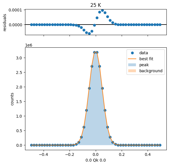
25 K Fit Results
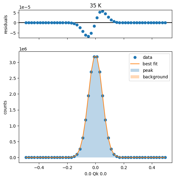
35 K Fit Results
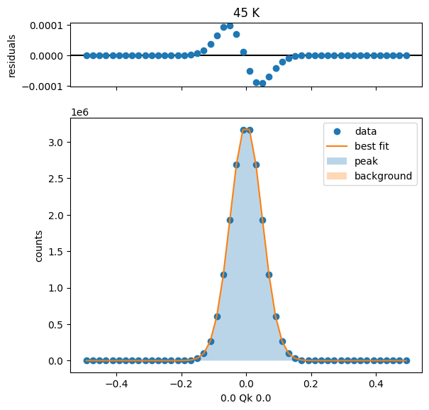
45 K Fit Results
55 K Fit Results

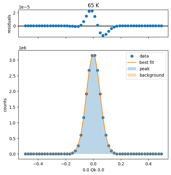
65 K Fit Results
75 K Fit Results
80 K Fit Results
104 K Fit Results

128 K Fit Results
153 K Fit Results

177 K Fit Results
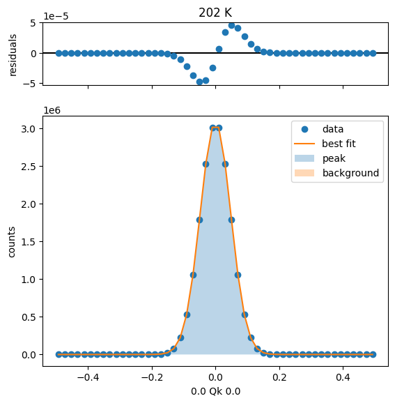
202 K Fit Results
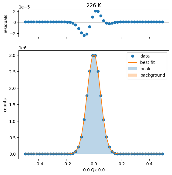
226 K Fit Results
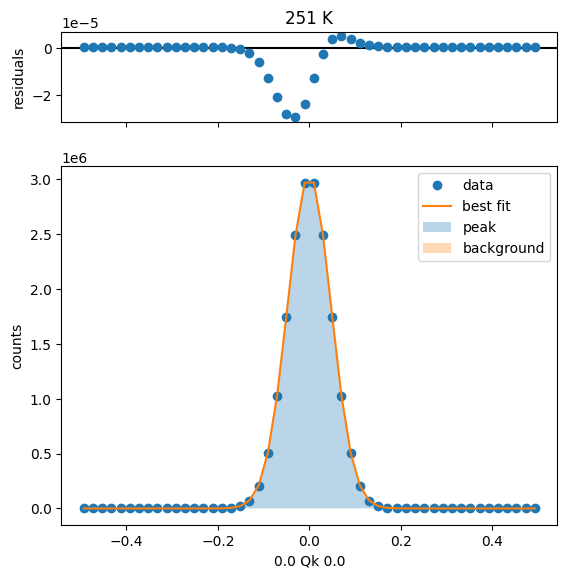
251 K Fit Results
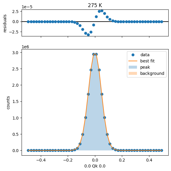
275 K Fit Results
300 K Fit Results

Overlay all fits
It can also be helpful to overlay the plots of all fits on a single figure. To accomplish this, we can use the .overlay_fits() method.
sample.overlay_fits()
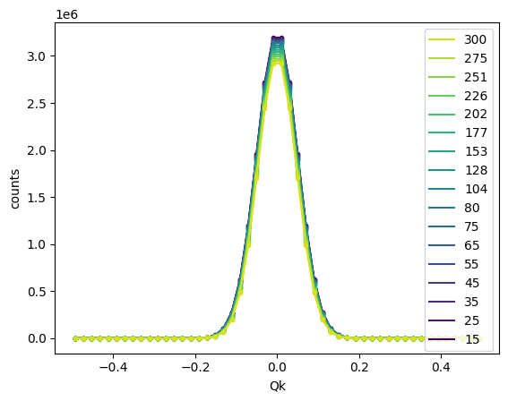
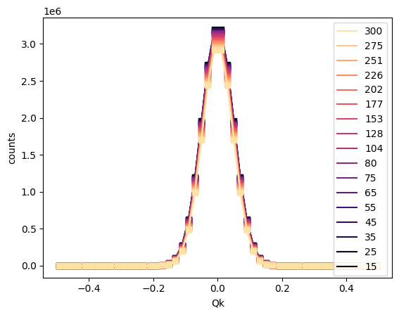
The numpoints parameter specifies the number of points to use for the fit curve. A vertical offset may be specified using vertical_offset for clarity. The colormap is also customizable via the cmap argument, and other customizations can be passed to the plot functions for the data and fit components via data_kwargs and fit_kwargs, respectively.
sample.overlay_fits(cmap='magma', data_kwargs={'marker':'s'})
/home/docs/checkouts/readthedocs.org/user_builds/nxs-analysis-tools/envs/stable/lib/python3.10/site-packages/nxs_analysis_tools/chess.py:749: UserWarning: marker is redundantly defined by the 'marker' keyword argument and the fmt string "." (-> marker='.'). The keyword argument will take precedence.
  ax.plot(lm.x, lm.y + vertical_offset * i, '.', c=colors[i], **data_kwargs)
Performing a simple linecut with no customization
The .fit_peak_simple() method offers a quick but rudimentary way to fit a peak, using a pseudo-Voigt peak shape with a linear background.
sample.fit_peak_simple()
sample.linecutmodels['15'].plot_fit()
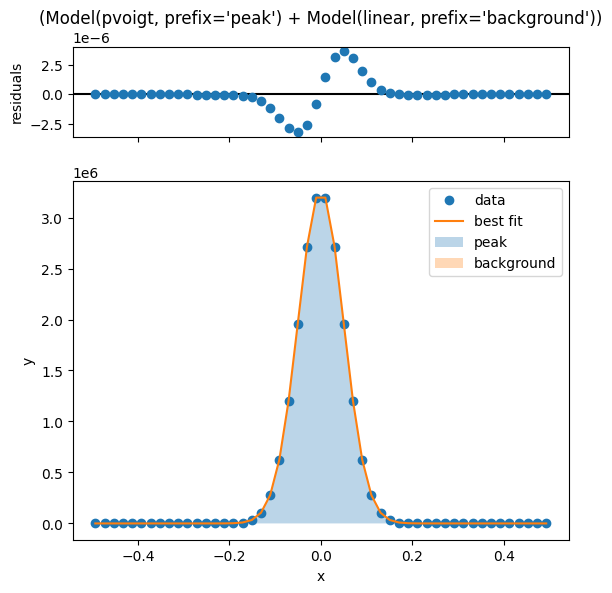
[[Model]]
    (Model(pvoigt, prefix='peak') + Model(linear, prefix='background'))
[[Fit Statistics]]
    # fitting method   = leastsq
    # function evals   = 239
    # data points      = 50
    # variables        = 6
    chi-square         = 7.1310e-11
    reduced chi-square = 1.6207e-12
    Akaike info crit   = -1351.80009
    Bayesian info crit = -1340.32795
    R-squared          = 1.00000000
##  Warning: uncertainties could not be estimated:
    peakcenter:           at initial value
    peakfraction:         at boundary
    backgroundslope:      at initial value
[[Variables]]
    peakamplitude:        407704.502 (init = 603160.9)
    peakcenter:          -8.6824e-14 (init = -7.401487e-17)
    peaksigma:            0.05872314 (init = 0.05033557)
    peakfraction:         3.0309e-13 (init = 0.5)
    peakfwhm:             0.11744628 == '2.0000000*peaksigma'
    peakheight:           3261174.43 == '(((1-peakfraction)*peakamplitude)/max(1e-15, (peaksigma*sqrt(pi/log(2))))+(peakfraction*peakamplitude)/max(1e-15, (pi*peaksigma)))'
    backgroundslope:      9.0210e-17 (init = 9.271793e-11)
    backgroundintercept: -9.1841e-12 (init = 404986.5)
<Axes: xlabel='x', ylabel='y'>