Visualizing CHESS temperature dependent data¶

Currently, there are two formats for CHESS data structures. The first was used prior to 2024, and was based on processing code written by Jacob Ruff. More recently, the beamline has switched to using nxrefine, a software plugin for NeXpy that allows for refinement of the scattering data.

Import functions¶

import matplotlib.pyplot as plt
from nxs_analysis_tools import TempDependence
from nxs_analysis_tools.datasets import cubic

sample_directory = cubic() # Download example data and store in cache directory

The `TempDependence` class¶

It is assumed that the folder structure of the temperature dependent scans is as follows:

samplename
└── labelname
    ├── 15
    ├── 100
    ├── 300
    ├── samplename_15.nxs
    ├── samplename_100.nxs
    ├── samplename_300.nxs

Here we create a TempDependence objecct called sample whose temperature folders are found in the path 'samplename/labelname/'. This can also be set separately using the .set_sample_directory() method.

sample = TempDependence(sample_directory)

Loading data¶

Option 1: Loading `nxrefine` processed data using `load_transforms()`¶

Use the load_transforms() method to load the “.nxs” files. All files ending with “.nxs” are imported.

sample.load_transforms()

data:NXdata
  @axes = ['Qh', 'Qk', 'Ql']
  @signal = 'counts'
  Qh = float64(100)
  Qk = float64(150)
  Ql = float64(200)
  counts = float64(100x150x200)
data:NXdata
  @axes = ['Qh', 'Qk', 'Ql']
  @signal = 'counts'
  Qh = float64(100)
  Qk = float64(150)
  Ql = float64(200)
  counts = float64(100x150x200)
data:NXdata
  @axes = ['Qh', 'Qk', 'Ql']
  @signal = 'counts'
  Qh = float64(100)
  Qk = float64(150)
  Ql = float64(200)
  counts = float64(100x150x200)
data:NXdata
  @axes = ['Qh', 'Qk', 'Ql']
  @signal = 'counts'
  Qh = float64(100)
  Qk = float64(150)
  Ql = float64(200)
  counts = float64(100x150x200)
data:NXdata
  @axes = ['Qh', 'Qk', 'Ql']
  @signal = 'counts'
  Qh = float64(100)
  Qk = float64(150)
  Ql = float64(200)
  counts = float64(100x150x200)
data:NXdata
  @axes = ['Qh', 'Qk', 'Ql']
  @signal = 'counts'
  Qh = float64(100)
  Qk = float64(150)
  Ql = float64(200)
  counts = float64(100x150x200)
data:NXdata
  @axes = ['Qh', 'Qk', 'Ql']
  @signal = 'counts'
  Qh = float64(100)
  Qk = float64(150)
  Ql = float64(200)
  counts = float64(100x150x200)
data:NXdata
  @axes = ['Qh', 'Qk', 'Ql']
  @signal = 'counts'
  Qh = float64(100)
  Qk = float64(150)
  Ql = float64(200)
  counts = float64(100x150x200)
data:NXdata
  @axes = ['Qh', 'Qk', 'Ql']
  @signal = 'counts'
  Qh = float64(100)
  Qk = float64(150)
  Ql = float64(200)
  counts = float64(100x150x200)
data:NXdata
  @axes = ['Qh', 'Qk', 'Ql']
  @signal = 'counts'
  Qh = float64(100)
  Qk = float64(150)
  Ql = float64(200)
  counts = float64(100x150x200)
data:NXdata
  @axes = ['Qh', 'Qk', 'Ql']
  @signal = 'counts'
  Qh = float64(100)
  Qk = float64(150)
  Ql = float64(200)
  counts = float64(100x150x200)
data:NXdata
  @axes = ['Qh', 'Qk', 'Ql']
  @signal = 'counts'
  Qh = float64(100)
  Qk = float64(150)
  Ql = float64(200)
  counts = float64(100x150x200)
data:NXdata
  @axes = ['Qh', 'Qk', 'Ql']
  @signal = 'counts'
  Qh = float64(100)
  Qk = float64(150)
  Ql = float64(200)
  counts = float64(100x150x200)
data:NXdata
  @axes = ['Qh', 'Qk', 'Ql']
  @signal = 'counts'
  Qh = float64(100)
  Qk = float64(150)
  Ql = float64(200)
  counts = float64(100x150x200)
data:NXdata
  @axes = ['Qh', 'Qk', 'Ql']
  @signal = 'counts'
  Qh = float64(100)
  Qk = float64(150)
  Ql = float64(200)
  counts = float64(100x150x200)
data:NXdata
  @axes = ['Qh', 'Qk', 'Ql']
  @signal = 'counts'
  Qh = float64(100)
  Qk = float64(150)
  Ql = float64(200)
  counts = float64(100x150x200)
data:NXdata
  @axes = ['Qh', 'Qk', 'Ql']
  @signal = 'counts'
  Qh = float64(100)
  Qk = float64(150)
  Ql = float64(200)
  counts = float64(100x150x200)

Option 2: Loading `3rot_hkli.nxs` files using `load_datasets()`¶

Use the load_datasets() method to load the “.nxs” files. By default, all files ending with “hkli.nxs” are imported, but this can be changed using the file_ending parameter.

# Method for loading legacy CHESS data format
# sample.load_datasets(file_ending="hkli.nxs")

A subset of temperatures can be imported using the temperatures_list parameter. Temperatures can be listed here as numeric values ([15,300]) or as strings (['15','300']).

sample.load_transforms(temperatures_list=[15,300])

# For legacy CHESS data format
# sample.load_datasets(temperatures_list=[15,300])

data:NXdata
  @axes = ['Qh', 'Qk', 'Ql']
  @signal = 'counts'
  Qh = float64(100)
  Qk = float64(150)
  Ql = float64(200)
  counts = float64(100x150x200)
data:NXdata
  @axes = ['Qh', 'Qk', 'Ql']
  @signal = 'counts'
  Qh = float64(100)
  Qk = float64(150)
  Ql = float64(200)
  counts = float64(100x150x200)

Similarly, select temperatures can be ignored during loading using the exclude_temperatures parameter.

sample.load_datasets(exclude_temperatures=[25])

Accessing the data¶

The datasets are stored under the .datasets attribute of the TempDependence object.

sample.datasets

{'15': NXdata('data'),
 '25': NXdata('data'),
 '35': NXdata('data'),
 '45': NXdata('data'),
 '55': NXdata('data'),
 '65': NXdata('data'),
 '75': NXdata('data'),
 '80': NXdata('data'),
 '104': NXdata('data'),
 '128': NXdata('data'),
 '153': NXdata('data'),
 '177': NXdata('data'),
 '202': NXdata('data'),
 '226': NXdata('data'),
 '251': NXdata('data'),
 '275': NXdata('data'),
 '300': NXdata('data')}

Use square brackets to index the individual datasets in the NXentry. Each dataset is a NXdata object and possesses the corresponding attributes and methods.

sample.datasets['15']

NXdata('data')

A list of temperatures is stored in the .temperatures attribute of the TempDependence object.

sample.temperatures

['15',
 '35',
 '45',
 '55',
 '65',
 '75',
 '80',
 '104',
 '128',
 '153',
 '177',
 '202',
 '226',
 '251',
 '275',
 '300']

Visualizing the data¶

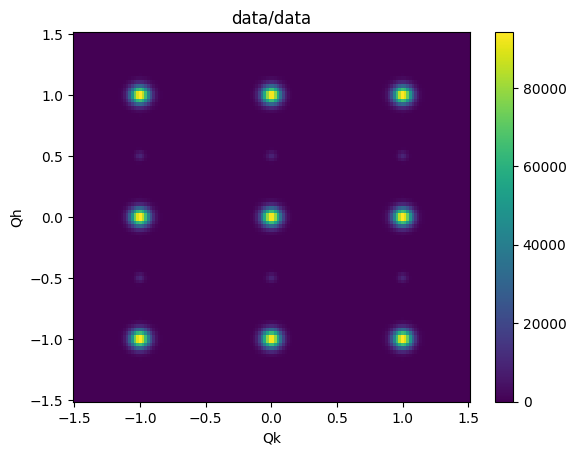
For example, each NXdata object has a .plot() method. Here we plot the L=0.0 plane.

sample.datasets['15'][:,:,0.0].plot()

../_images/9743f79c7039916039c78bf10ad40c8800564c20aec4b4fa1cd5a9709e929937.png

Temperature dependent linecuts¶

Linecuts are performed using the Scissors class. An instance of the Scissors class is created for each temperature and stored in a dict attribute called scissors.

See documentation on the Scissors class for more information.

sample.scissors

{'15': <nxs_analysis_tools.datareduction.Scissors at 0x790a8026a950>,
 '25': <nxs_analysis_tools.datareduction.Scissors at 0x790a802e2ad0>,
 '35': <nxs_analysis_tools.datareduction.Scissors at 0x790a802c4520>,
 '45': <nxs_analysis_tools.datareduction.Scissors at 0x790a802c6a10>,
 '55': <nxs_analysis_tools.datareduction.Scissors at 0x790a802c6890>,
 '65': <nxs_analysis_tools.datareduction.Scissors at 0x790a827c5fc0>,
 '75': <nxs_analysis_tools.datareduction.Scissors at 0x790ab8321210>,
 '80': <nxs_analysis_tools.datareduction.Scissors at 0x790ab8323eb0>,
 '104': <nxs_analysis_tools.datareduction.Scissors at 0x790ab83212d0>,
 '128': <nxs_analysis_tools.datareduction.Scissors at 0x790ab8321450>,
 '153': <nxs_analysis_tools.datareduction.Scissors at 0x790a802e2e00>,
 '177': <nxs_analysis_tools.datareduction.Scissors at 0x790a802e2e60>,
 '202': <nxs_analysis_tools.datareduction.Scissors at 0x790a802e2ec0>,
 '226': <nxs_analysis_tools.datareduction.Scissors at 0x790a802e2f20>,
 '251': <nxs_analysis_tools.datareduction.Scissors at 0x790a802e2f80>,
 '275': <nxs_analysis_tools.datareduction.Scissors at 0x790a802e2fe0>,
 '300': <nxs_analysis_tools.datareduction.Scissors at 0x790a802e3040>}

The individual Scissors objects can be indexed using square brackets and the temperature.

sample.scissors['15']

<nxs_analysis_tools.datareduction.Scissors at 0x790a8026a950>

Batch linecuts are peformed using a method of the TempDependence class called .cut_data(), which internally calls the .cut_data() method on each of the Scissors objects at each temperature.

# First, load all available temperatures
sample.load_transforms()

# Perform the linecut
sample.cut_data(center=(0,0,0), window=(0.75,0.2,0.1))

data:NXdata
  @axes = ['Qh', 'Qk', 'Ql']
  @signal = 'counts'
  Qh = float64(100)
  Qk = float64(150)
  Ql = float64(200)
  counts = float64(100x150x200)
data:NXdata
  @axes = ['Qh', 'Qk', 'Ql']
  @signal = 'counts'
  Qh = float64(100)
  Qk = float64(150)
  Ql = float64(200)
  counts = float64(100x150x200)
data:NXdata
  @axes = ['Qh', 'Qk', 'Ql']
  @signal = 'counts'
  Qh = float64(100)
  Qk = float64(150)
  Ql = float64(200)
  counts = float64(100x150x200)
data:NXdata
  @axes = ['Qh', 'Qk', 'Ql']
  @signal = 'counts'
  Qh = float64(100)
  Qk = float64(150)
  Ql = float64(200)
  counts = float64(100x150x200)
data:NXdata
  @axes = ['Qh', 'Qk', 'Ql']
  @signal = 'counts'
  Qh = float64(100)
  Qk = float64(150)
  Ql = float64(200)
  counts = float64(100x150x200)
data:NXdata
  @axes = ['Qh', 'Qk', 'Ql']
  @signal = 'counts'
  Qh = float64(100)
  Qk = float64(150)
  Ql = float64(200)
  counts = float64(100x150x200)
data:NXdata
  @axes = ['Qh', 'Qk', 'Ql']
  @signal = 'counts'
  Qh = float64(100)
  Qk = float64(150)
  Ql = float64(200)
  counts = float64(100x150x200)
data:NXdata
  @axes = ['Qh', 'Qk', 'Ql']
  @signal = 'counts'
  Qh = float64(100)
  Qk = float64(150)
  Ql = float64(200)
  counts = float64(100x150x200)
data:NXdata
  @axes = ['Qh', 'Qk', 'Ql']
  @signal = 'counts'
  Qh = float64(100)
  Qk = float64(150)
  Ql = float64(200)
  counts = float64(100x150x200)
data:NXdata
  @axes = ['Qh', 'Qk', 'Ql']
  @signal = 'counts'
  Qh = float64(100)
  Qk = float64(150)
  Ql = float64(200)
  counts = float64(100x150x200)
data:NXdata
  @axes = ['Qh', 'Qk', 'Ql']
  @signal = 'counts'
  Qh = float64(100)
  Qk = float64(150)
  Ql = float64(200)
  counts = float64(100x150x200)
data:NXdata
  @axes = ['Qh', 'Qk', 'Ql']
  @signal = 'counts'
  Qh = float64(100)
  Qk = float64(150)
  Ql = float64(200)
  counts = float64(100x150x200)
data:NXdata
  @axes = ['Qh', 'Qk', 'Ql']
  @signal = 'counts'
  Qh = float64(100)
  Qk = float64(150)
  Ql = float64(200)
  counts = float64(100x150x200)
data:NXdata
  @axes = ['Qh', 'Qk', 'Ql']
  @signal = 'counts'
  Qh = float64(100)
  Qk = float64(150)
  Ql = float64(200)
  counts = float64(100x150x200)
data:NXdata
  @axes = ['Qh', 'Qk', 'Ql']
  @signal = 'counts'
  Qh = float64(100)
  Qk = float64(150)
  Ql = float64(200)
  counts = float64(100x150x200)
data:NXdata
  @axes = ['Qh', 'Qk', 'Ql']
  @signal = 'counts'
  Qh = float64(100)
  Qk = float64(150)
  Ql = float64(200)
  counts = float64(100x150x200)
data:NXdata
  @axes = ['Qh', 'Qk', 'Ql']
  @signal = 'counts'
  Qh = float64(100)
  Qk = float64(150)
  Ql = float64(200)
  counts = float64(100x150x200)

{'15': NXdata('data'),
 '25': NXdata('data'),
 '35': NXdata('data'),
 '45': NXdata('data'),
 '55': NXdata('data'),
 '65': NXdata('data'),
 '75': NXdata('data'),
 '80': NXdata('data'),
 '104': NXdata('data'),
 '128': NXdata('data'),
 '153': NXdata('data'),
 '177': NXdata('data'),
 '202': NXdata('data'),
 '226': NXdata('data'),
 '251': NXdata('data'),
 '275': NXdata('data'),
 '300': NXdata('data')}

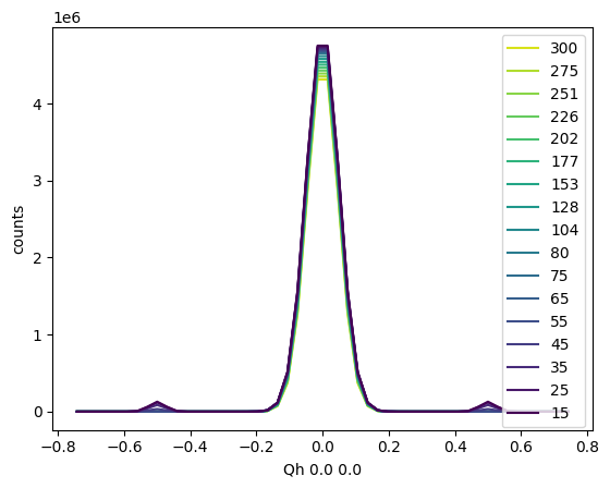
Similarly, batch plotting of the linecuts can be achieved using the .plot_linecuts() method of the TempDependence object, which internally calls the .plot_linecut() method of the Scissors objects at each temperature.

sample.plot_linecuts()

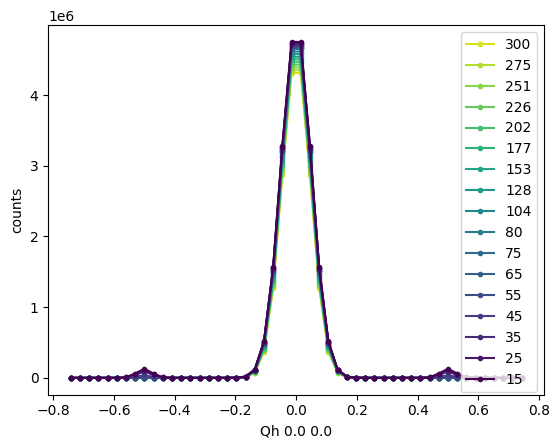
../_images/01a6cc183d2f3690144dc43612a2f5b4a995e92110ddbf2f5d84d084edec5883.png

Any keyword arguments are passed to a matplotlib function ax.plot() within .plot_linecuts(), so the usual matplotlib parameters can be used to change the formatting.

sample.plot_linecuts(linestyle='-', marker='.')

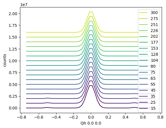
../_images/c69efc0166c7fce731879528772982cfa08b8f1e9c0d738a1610a0bdbce56607.png

You can also introduce a vertical offset using the vertical_offset parameter.

sample.plot_linecuts(vertical_offset=1e6)

../_images/26748c77e91d7fb89f1207a0a3ed867f2c21efea3f9427cbceb59c93ee5fe0db.png

Visualizing the integration window¶

To visualize where the integration was performed, use the .plot_integration_window() method of the Scissors class.

sample.scissors['15'].plot_integration_window()

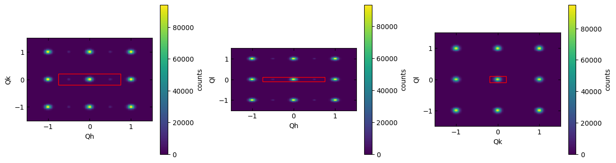
../_images/54ddf7b98e038d3ee0416fa90815f11cee7bb6bfeaee8bcd513af247147102a2.png

(<matplotlib.collections.QuadMesh at 0x790a68db5ab0>,
 <matplotlib.collections.QuadMesh at 0x790a68e9f3d0>,
 <matplotlib.collections.QuadMesh at 0x790a67d2c220>)

Use the optional width and height parameters to zoom in on the region of interest.

sample.scissors['15'].plot_integration_window(width=1.5, height=0.5)

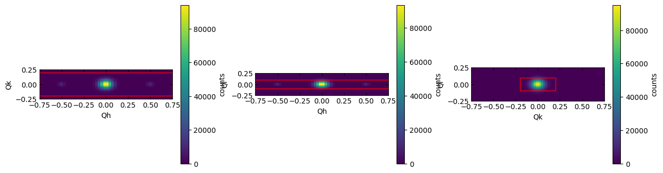
../_images/64a3f6d75f55be023aacaecb0efb08a77a49ac35a413f9be5710fefbc2f63e23.png

(<matplotlib.collections.QuadMesh at 0x790a6904ea40>,
 <matplotlib.collections.QuadMesh at 0x790a6917afb0>,
 <matplotlib.collections.QuadMesh at 0x790a691f8760>)