Extracting Delta-PDF maps from diffuse scattering

from nxs_analysis_tools import *
from nxs_analysis_tools.datasets import vacancies
from nxs_analysis_tools.datareduction import load_discus_nxs

data_path = vacancies()

import matplotlib.pyplot as plt

Downloading file 'vacancies.nxs' from 'https://raw.githubusercontent.com/stevenjgomez/dataset-vacancies/main/vacancies.nxs' to '/home/docs/.cache/nxs_analysis_tools/vacancies'.

Here we showcase the use of the DeltaPDF class found in the pairdistribution module of the nxs-analysis-tools package. For the example data, we consider a model structure of Cu where there are 3% vacancies. These vacancies cause the surrounding atoms along the 100-type directions to relax by 15% of the interatomic spacing towards the vacancy. A representative plane is shown below:

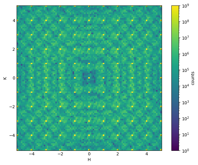
Visualizing the diffuse scattering data

First let’s load the example dataset:

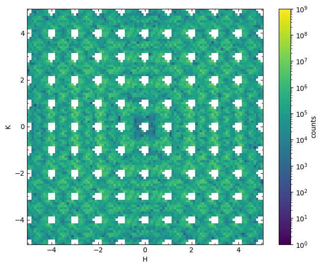
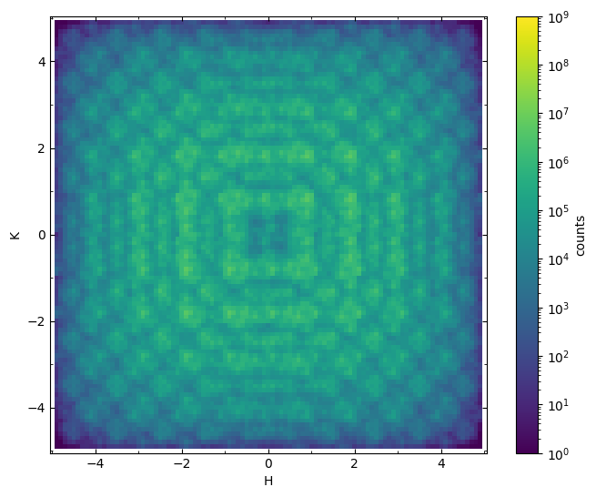
data = load_discus_nxs(data_path)

plot_slice(data[:,:,0.0], vmin=1, vmax=1e9, logscale=True)

<matplotlib.collections.QuadMesh at 0x7a1a19ddffd0>

Importing the DeltaPDF class

Clearly, there is evidence for diffuse scattering in the background of the usual Bragg reflections. This is the perfect use case to apply the DeltaPDF technique. To facilitate this, we import the DeltaPDF object:

from nxs_analysis_tools.pairdistribution import DeltaPDF

We’ll initialize an object called dpdf which will be an instance of the DeltaPDF class, allowing us to use the tools stored in this class.

dpdf = DeltaPDF()

Step 1: Setup the data and lattice information

First, we set the data to be transformed:

dpdf.set_data(data)

Next, we set the lattice parameters. Here we assume a cubic cell with lattice parameter of 5 Angstroms.

dpdf.set_lattice_params((5,5,5,90,90,90))

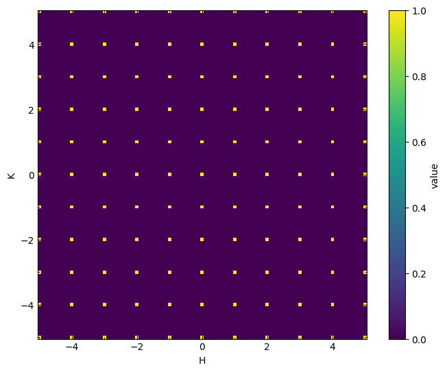
Step 2: Generate a mask for Bragg peaks and unwanted pixels

For removal of well-defined Bragg peaks, one can usually create a mask of spheres or ellipsoids around the integer Bragg positions. This can be done using the .generate_bragg_mask() method.

First, we examine the case of spheres around each integer coordinate. Simply specify a punch_radius in lattice units to remove from the dataset, and a mask will be generated accordingly.

mask = dpdf.generate_bragg_mask(punch_radius=0.2)

Let’s visualize a cross section of the mask:

plot_slice(mask[:,:,mask.shape[2]//2], data.H, data.K)

# Set aspect ratio to the lattice parameter ratio b/a
plt.gca().set_aspect(dpdf.lattice_params[1]/dpdf.lattice_params[0])

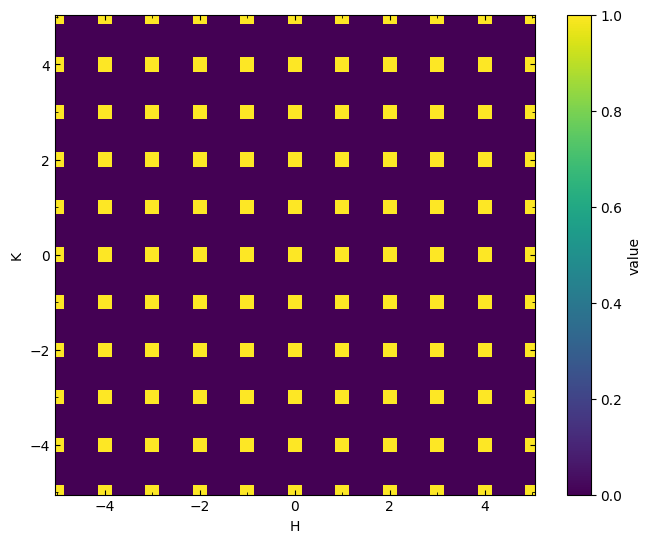
Sometimes it is useful to create ellipsoids rather than spheres. For this purpose, you may specify coefficients using the coeffs parameter to modify the H^2, HK, K^2, KL, L^2, and LH terms of the ellipsoid equation, respectively. The default is coeffs=[1,0,1,0,1,0] (i.e., no cross terms). If I want to create an ellipsoid that is elongated along the K axis, I can do so by changing the coefficients as follows:

mask = dpdf.generate_bragg_mask(punch_radius=0.2, coeffs=[1,0,0.4,0,1,0])
plot_slice(mask[:,:,mask.shape[2]//2], data.H, data.K)
plt.gca().set_aspect(dpdf.lattice_params[1]/dpdf.lattice_params[0])

Likewise, if I need the ellipsoids to elongate diagonally, I can add a non-zero cross term in the HK direction.

mask = dpdf.generate_bragg_mask(punch_radius=0.2, coeffs=[1,1,1,0,1,0])
plot_slice(mask[:,:,mask.shape[2]//2], data.H, data.K)
plt.gca().set_aspect(dpdf.lattice_params[1]/dpdf.lattice_params[0])

In addition, the thresh parameter can be used to define a threshold intensity within these ellipsoids, such that pixels below this threshold are kept and pixels above the threshold are removed. For example:

mask = dpdf.generate_bragg_mask(punch_radius=0.2, thresh=1e9)
plot_slice(mask[:,:,mask.shape[2]//2], data.H, data.K)
plt.gca().set_aspect(dpdf.lattice_params[1]/dpdf.lattice_params[0])

Another option for masking pixels is to use the .generate_intensity_mask() method to mask out ALL pixels above a certain threshold, including a small chosen radius (in px) of surrounding pixels.

mask = dpdf.generate_intensity_mask(thresh=1e9, radius=1)
plot_slice(mask[:,:,mask.shape[2]//2], data.H, data.K)
plt.gca().set_aspect(dpdf.lattice_params[1]/dpdf.lattice_params[0])

Shape of data is (101, 101, 101)
Found high intensity at 1331 individual points.
Done.

Lastly, there is the option to generate an ellipsoid as described earlier, but at a general coordinate using .generate_mask_at_coord().

mask = dpdf.generate_mask_at_coord(coordinate=(2,0,0), punch_radius=0.5)
plot_slice(mask[:,:,mask.shape[2]//2], data.H, data.K)
plt.gca().set_aspect(dpdf.lattice_params[1]/dpdf.lattice_params[0])

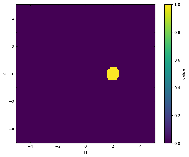
The same coeffs and thresh can be specified for this method as well.

To formally set the mask to use for the punching operation, one must use the .add_mask() method. This can be used in conjunction with the.subtract_mask() method to generate complex and custom masks.

For now, we will use the standard Bragg mask of spheres around each Bragg reflection.

mask = dpdf.generate_bragg_mask(punch_radius=0.2)
dpdf.add_mask(mask)

To apply the mask to the data, use the .punch() method.

dpdf.punch()

The punched data is then stored in the .punched attribute.

plot_slice(dpdf.punched[:,:,0.0], vmin=1, vmax=1e9, logscale=True)

<matplotlib.collections.QuadMesh at 0x7a1a0fbac160>

Step 3: Fill in missing data

Filling in the resulting gaps in the data requires convolution with a Gaussian kernel, effectively interpolating the missing data using surrounding values.

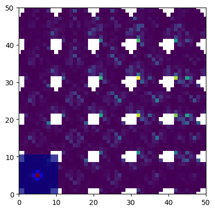
First, we set a kernel using the .set_kernel() method. Here we call the built-in Gaussian3DKernel function, which provides a 3D Gaussian shape that can be modified using the coeffs parameter to become an ellipsoid as described above. Here we choose a standard deviation of 1 and a size of 10x10x10 cubic pixels.

from nxs_analysis_tools.pairdistribution import Gaussian3DKernel
dpdf.set_kernel(Gaussian3DKernel(stddev=1, size=(10,10,10)))                                                                                                           

It may be insightful at this point to visualize the kernel to get an idea for its size relative to the dataset. Use the imshow function from matplotlib to get an apples-to-apples comparison of the dimensions of these two objects.

fig,ax = plt.subplots() # Create a common figure and axes to plot on
ax.imshow(dpdf.punched[:,:,0.0].nxsignal.nxdata, cmap='viridis') # Plot the punched data
ax.imshow(dpdf.kernel.array[:,:,dpdf.kernel.array.shape[2]//2], alpha=0.75, cmap='jet') # Plot a cross section of the kernel
ax.set(xlim=(0,50), ylim=(0,50)) # Zoom into the corner where the kernel is plotted

[(0.0, 50.0), (0.0, 50.0)]

To perform the interpolation, use the .interpolate() method.

dpdf.interpolate()

Running interpolation...
Interpolation finished.
Interpolation took 0.00 minutes.

The results are stored in the .interpolated attribute:

plot_slice(dpdf.interpolated[:,:,0.0], vmin=1, vmax=1e9, logscale=True)

<matplotlib.collections.QuadMesh at 0x7a1a0e3ac3d0>

Step 4: Taper edges of data

Now that we have successfully isolated the diffuse scattering, the edges of the data must be tapered to a zero value in order to avoid cutoff artifacts (ripples) after the Fourier transform.

Three built-in options for tapering windows are provided: .set_tukey_window(), .set_ellipsoidal_tukey_window(), and .set_hexagonal_tukey_window(). The first applies a standard tukey window from the scipy package along H, K, and L, the second applies a radial taper resulting in an ellipsoidal window, and the third applies a hexagonal tukey window in the HK plane and a standard tukey window along L.

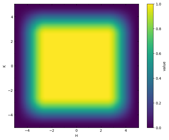
dpdf.set_tukey_window()

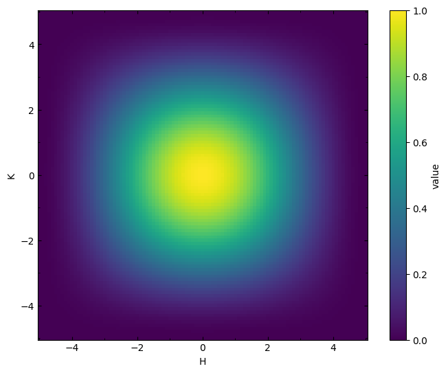
The chosen window is stored in the .window attribute:

plot_slice(dpdf.window[:,:,data.shape[2]//2], data.H, data.K, vmin=0, vmax=1)

<matplotlib.collections.QuadMesh at 0x7a1a0fb20880>

The optional tukey_alphas parameter allows the user to provide a tuple of values for the tukey alpha to be applied along each direction. For the .set_tukey_window() method, a three-tuple should be provided (e.g., (0.5,0.5,0.5)) corresponding to H, K, and L directions. For the .set_hexagonal_tukey_window(), a four-tuple should be provided (e.g., (0.5,0.5,0.5,0.5)) corresponding to H, K, HK, and L directions.

dpdf.set_tukey_window(tukey_alphas=(0.5,0.5,0.5))

plot_slice(dpdf.window[:,:,data.shape[2]//2], data.H, data.K, vmin=0, vmax=1)

<matplotlib.collections.QuadMesh at 0x7a1a14060a30>

To apply the window to the data, use the .apply_window() method.

dpdf.set_tukey_window()
dpdf.apply_window()

The resulting tapered data is stored in the .tapered attribute.

plot_slice(dpdf.tapered[:,:,0.0], vmin=1, vmax=1e9, logscale=True)

<matplotlib.collections.QuadMesh at 0x7a1a141fde70>

Step 5: Pad data with zeros

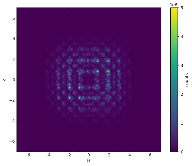
Lastly, in order to improve the resolution of the pdf after the Fourier transform, we must pad the data with zeros around the original reciprocal space volume using the .pad() method. The padding parameter allows the user to provide a tuple of three integers to specify the number of pixels add to each side along the H, K, and L directions.

dpdf.pad(padding=(20,20,20))

The padded data is stored in the .padded attribute

plot_slice(dpdf.padded[:,:,0.0], vmin=0, vmax=5e6, logscale=False)

<matplotlib.collections.QuadMesh at 0x7a1a0e0375e0>

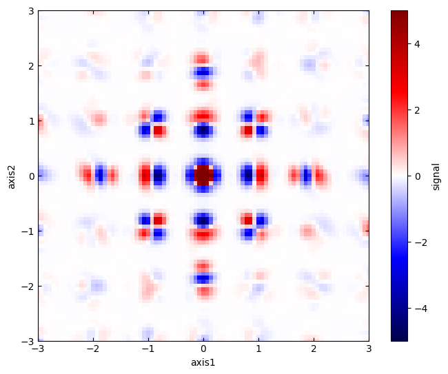
Step 6: Perform Fourier transform

Use the .perform_fft() method to begin running the Fourier transform.

dpdf.perform_fft()

FFT started.
Performing FFT...
FFT completed in 1.159 seconds.

/home/docs/checkouts/readthedocs.org/user_builds/nxs-analysis-tools/envs/stable/lib/python3.10/site-packages/nxs_analysis_tools/pairdistribution.py:1513: UserWarning: In version v0.1.15 and beyond, the default method was changed from method='staged' to method='complete' to avoid issues with data containing a non-orthogonal third coordinate axis. Previous behavior can be restored by using method='staged'.
  warnings.warn(

The resulting 3D-DeltaPDF is stored in the .fft attribute.

plot_slice(dpdf.fft[:,:,0.0]/1e3, cmap='seismic',
           vmin=-5, vmax=5,
           xlim=(-3,3),
           ylim=(-3,3),
          )

<matplotlib.collections.QuadMesh at 0x7a1a0e23d150>